Using Query APIs to Unlock the Power of Azure Time Series Insights Part 2: The Aggregates APIs
 By Basim Majeed, Cloud Solution Architect at Microsoft
This is the second part of the blog series which aims to clarify the query APIs of Azure Time Series Insights (TSI) by the use of examples. It is recommended that you visit the first part of this series in order to learn more about how to set up the TSI environment and how to use Postman to replicate and modify the examples we show here.
In the example we are using here, the message sent by the simulated device is of the following JSON format:
{"tag":"Pres_22","telemetry":"Pressure","value":12.02848,"factory":"Factory_2","station":"Station_2"}
We have two types of telemetry; Temperature and Pressure. The data represents a simple industrial environment with 2 factories, 2 stations per factory and two sensors for each station measuring Temperature and Pressure. For simplicity, all the data is channelled through one IoT device (iotDevice_1) connected to the to the IoT Hub, though you might want to have many devices connected directly to the Hub.
In this blog we focus our attention on the Aggregates API, which provides the capability to group events by a given dimension and to measure the values of other properties using aggregate expressions, which apply to the property types “Double” and “DateTime”. For the properties of “Double” we can use “min”, “max”, “avg” and “sum” expressions, while for “DateTime” we can only use the “min” and “max” expressions. The dimensions that we can use to group the events are "uniqueValues", "dateHistogram" and "numericHistogram".
Building the Aggregate query
You start an aggregate query by defining a “searchSpan” to determine the time period over which the data is collected. Then you need to build the “aggregates” clause of the query, within which you need to define the “uniqueValues” dimension that determines the grouping of data. For example, if you group by a “sensorID” then all the following calculations will be done for each unique value of “sensorID”. To limit the number of unique values returned you need to use a “take” or “sample” clause, as will be shown in the examples.
Next, still within the “aggregates” clause, you need to decide on the property you want to return an aggregate measure for. As an example, you could choose to calculate the minimum value of a property over the full “searchSpan”.
All the requests in the following examples are directed to the “aggregates” resource path as explained in part 1 of this blog series:
POST https://<environmentFqdn>/aggregates?api-version=<apiVersion>
Example 1: Return the minimum, maximum and average sensor readings
In this example we return the average, minimum and maximum readings for each unique sensor tag value over the defined time period defined by the “searchSpan” clause. We are limiting the number of sensors that we will apply the aggregate calculation to by using the “take” clause, in this case set to 10 sensors. Since we only have 8 sensor tags in the data sample then all the tags will be returned in the response. If, for example, the “take” clause defined a value of 4, only 4 sensor tags will be used for the aggregation. Note that the use of “take” returns property values without any particular order. The response is shown in Figure 1.
Request Body
 {
    "searchSpan": {
        "from": { "dateTime":"{{startdate}}" },
        "to": { "dateTime":"{{enddate}}" }
    },
    "aggregates": [
        {
            "dimension": {
                "uniqueValues": {
                    "input": { "property": "tag", "type": "String" },
                    "take": 10
                }
            },
            "measures": [
                {
                    "avg": {
                        "input": { "property": "value", "type": "Double" }
                    }
                },
                {
                    "min": {
                        "input": { "property": "value", "type": "Double" }
                    }
                },
                {
                    "max": {
                        "input": { "property": "value", "type": "Double" }
                    }
                }
            ]
        }
    ]
}
Response Body
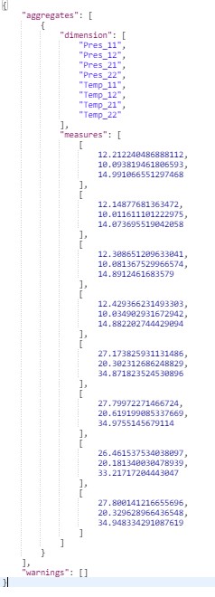
Figure 1: The average, minimum and maximum values per sensor tag
Example 2: Using “predicate” to restrict the dimensions based on a condition
If we want to be more specific about the “dimension”, we can insert a “predicate” clause before the “aggregates” clause. We want to limit the sensors selected for the aggregation dimensions to only those that provide the temperature telemetry. This is done using the equality expression “eq”. Note also that we are only choosing to return the results for 2 sensors as specified by the “take” clause. The response is shown in Figure 2.
POST https://<environmentFqdn>/aggregates?api-version=<apiVersion>
Request Body
 {
    "searchSpan": {
        "from": { "dateTime":"{{startdate}}" },
        "to": { "dateTime":"{{enddate}}" }
    },
    "predicate":{
        "eq": {
            "left": {
                "property": "telemetry",
                    "type": "String"
            },
            "right": "Temperature"
        }
    },
    "aggregates": [
        {
            "dimension": {
                "uniqueValues": {
                    "input": { "property": "tag", "type": "String" },
                    "take": 2
                }
            },
            "measures": [
                {
                    "avg": {
                        "input": { "property": "value", "type": "Double" }
                    }
                },
                {
                    "min": {
                        "input": { "property": "value", "type": "Double" }
                    }
                },
                {
                    "max": {
                        "input": { "property": "value", "type": "Double" }
                    }
                }
            ]
        }
    ]
}
Response Body
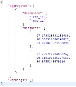
Figure 2: The effect of the “predicate” clause on the query response
Example 3: Using the date histogram
In this example we take a look at how to report a measure using a date histogram, i.e. by dividing the time axis into a number of fixed buckets and reporting the measure(s) over each individual bucket.
We start the query as usual by defining the “searchSpan”, and we also use the “predicate” clause to restrict our data to that coming from the temperature sensors. We then start the “aggregates” clause and choose the “tag” property as our “uniqueValues” dimension so the histogram calculations will be per “tag”. The “take” clause limits the number of tags considered here to two only. The “dateHistogram” is a dimension in itself and thus it needs to be defined inside an inner “aggregate” clause (note the difference between the outer “aggregates” and the inner “aggregate” clauses).
We define the “dateHistogram” by two properties. The first one is the “input” property which defines the time axis for the histogram, and in this case we use the built-in time variable “$ts” (the $ts property is generated by the TSI event ingestion process based on the information from the event source, e.g IoT hub, and can be replaced by another property that represents the time axis if required as long as it is defined as part of the event). The second property is the “breaks” property which defines the time duration of each of the buckets we need to report against. In this case we are dividing the time axis into 20 minute intervals.
We also need the “measures” definition inside the “aggregate” clause. Notice that we have included two measures in this case; the average value of the temperature (defined by the “avg” clause) and the number of values of temperature readings within each interval (defined by the “count” clause). So in this example we have combined two “dimension” properties together to produce the histogram; the “uniqueValues” and the “dateHistogram” dimensions. The results are shown in Figure 3.
Request Body
 {
    "searchSpan": {
        "from": { "dateTime":"{{startdate}}" },
        "to": { "dateTime":"{{enddate}}" }
    },
    "predicate":{
        "eq": {
            "left": {
                "property": "telemetry",
                    "type": "String"
            },
            "right": "Temperature"
        }
    },
    "aggregates": [
        {
            "dimension": {
                "uniqueValues": {
                    "input": { "property": "tag", "type": "String" },
                    "take": 2
                }
            },
            "aggregate": {
                "dimension": {
                    "dateHistogram": {
                        "input": { "builtInProperty": "$ts" },
                        "breaks": { "size": "20m" }
                    }
                },
                "measures": [
                    {
                        "avg": {
                            "input": { "property": "value", "type": "Double" }
                        }
                    },
                    {
                        "count": {}
                    }
                ]
            }
        }
    ]
}
Response Body
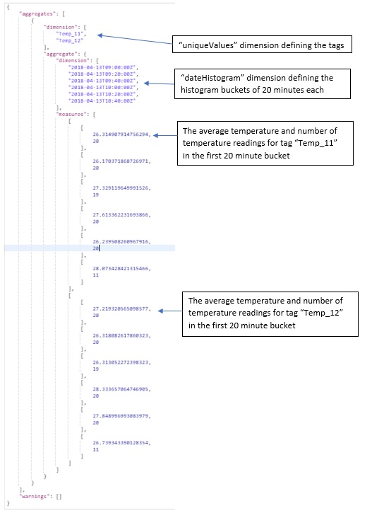
Figure 3: Results for the “dateHistogram”
Example 4: Using the numeric histogram
The numeric histogram is used to report the measure (e.g. the count) against value intervals. For example, if we have a sensor reporting some measurement in the range of 10 to 15, we can divide this range into a number of value buckets (10-11, 11-12, and so on). Then we can measure the number of events coming within each range. The way we construct the query is similar to the previous example apart from replacing “dateHistogram” with “numericHistogram”, and then defining how many value intervals we need in the “breaks” clause.
The TSI documentation states that “For numeric histogram, bucket boundaries are aligned to one of 10^n, 2x10^n or 5x10^n values”. So, if we have sensor data that ranges in values between 10 and 15 such as in the Pressure sensor of this example, we can choose 5 buckets of size 1, or 3 buckets of size 2, or 50 bucket of size 0.1 and so on, but we cannot have buckets of size 0.25 or 0.3 etc. We can only set the value of the “breaks” in the query but not the value of the bucket size. TSI will work out the sizer of buckets accordingly.
For the range of 10-15 that we have here, if we choose “breaks” to be 5 then we will get 5 buckets of size 1 each, however if we ask for 15 buckets then we will only get back 10 buckets of size of 0.5 each. The results are shown in Figure 4 for the cases “breaks” set to 5 and 15.
Request Body
 {
    "searchSpan": {
        "from": { "dateTime":"{{startdate}}" },
        "to": { "dateTime":"{{enddate}}" }
    },
    "predicate":{
        "eq": {
            "left": {
                "property": "telemetry",
                    "type": "String"
            },
            "right": "Pressure"
        }
    },
    "aggregates": [
        {
            "dimension": {
                "uniqueValues": {
                    "input": { "property": "tag", "type": "String" },
                    "take": 1
                }
            },
            "aggregate": {
                "dimension": {
                    "numericHistogram": {
                        "input": {
                            "property": "value",
                            "type": "Double"
                        },
                        "breaks": {
                            "count": 5
                        }
                    }
                },
                "measures": [
                    {
                        "count": {}
                    }
                ]
            }
        }
    ]
}
Response Body
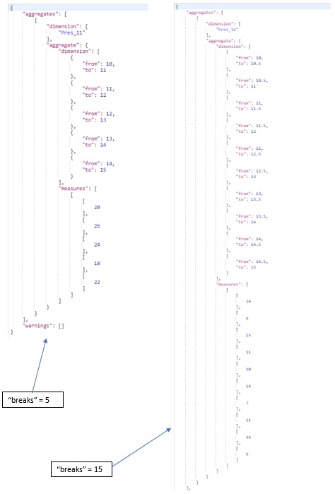
Figure 4: The “numericHistogram” results
Conclusions
The examples we explored here show the power of the aggregation APIs within Azure Time Series Insights in summarising events data and thus providing a way for users to build custom analytics that focus on their specific requirements. In the third part of this blog series we will look at more query capabilities within the TSI APIs.
---
Be sure to check out part 3! Basim takes a look at how you can use the predicate string as a way to define our query predicate in a much more human readable and understandable way.