Three Models for Anomaly Detection: Pros and Cons

Continuing the previous research on Machine Learning: Achieving Ultimate Intelligence, SoftServe’s Data Science Group (DSG) describes informational security risk identification by detecting deviations from the typical pattern of network activity.

The models that will be looked at are the Dynamic Threshold Model, the Association Rules Based Model, and the Time Series Clustering Model.

By Tetiana Gladkikh , Taras Hnot and Volodymyr Solskyy

What lies at the heart of a Dynamic Threshold Model is representation of a user's activity, expressed as a set of measured parameter values (metrics) for a certain observation category through a time series. It allows the establishment of presence or absence of general tendencies that can be expressed in the form of a general trend or have a seasonal character. For example, we can consider a time series that reflects a week of network activity of group members through the total amount of data transmitted in one minute (Fig. 1).

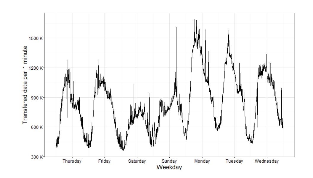
Fig. 1. Time Series Example

There is a common trend within this time section: through the week the average user activity decreases. At the same time, the process cannot be considered as proportional: there is a periodic sequence related to the fact that the maximum and minimum activity fits in the middle of the employees’ work day and night-time correspondingly. In this way each day’s activity can be described by a common pattern with minor amendments from the primary trend. User activity may then be described in the form of a discrete time series (signal quantized in both time and amplitude), along with evaluating a potential sampling error (allowed deviation threshold) (fig. 2). If the replacement analogue signal with a discrete error exceeds the permitted deviation threshold, the situation can be evaluated as an anomaly.

The next step is setting the maximum network load threshold for each part of the time series. The main reasoning behind this is to have average user activity reflected in both series trending and seasonal components, with the changes in load behaviour taken into account.

The model shown allows the description of user activity in the network through a limited set of constants. This set can be obtained at the initial stage of system adjustment and doesn’t require the entire set of historical data analysis "on the fly" to operate.

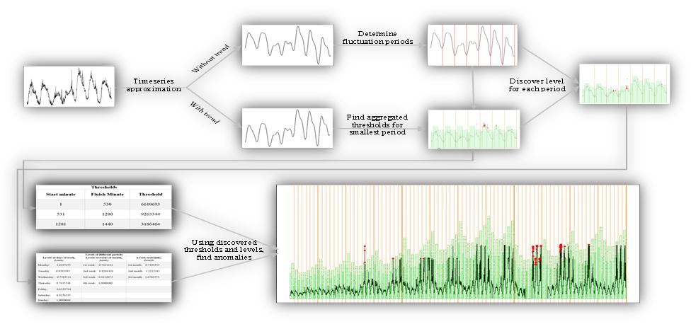
Fig. 2. Flow of Anomaly Detection based on user activity

In addition, the model may be easily adapted to the changing process. If significant deviations of the discrete time series from the continuous one become more frequent, it is enough to merely adjust the threshold values and/or coefficients of the relative load.

Association Rules Based Model

As mentioned before, the process being monitored can be represented as a set of linked events. Speaking about the activity of the user and/or group of users in the network, consider a single metric one-time value calculated for the category and/or a several categorical variables combination. For example, for sampling step time in 1 minute, estimate a total number of transmitted packets by a department for 1 minute on a TCP/IP protocol in the first half of the work day and at the same time estimate the total amount of packets via UDP protocol for the same user group.

We are not really interested in the absolute value of each of these categories, but rather in the relative number of cases when this activity was recorded.

For example, let’s take a time series which reflects a needed parameter change in time. In most cases, the results of this measurement will be presented by a continuous variable, i.e. it takes an infinite number of values. Each value is unique within a quantization scale, which makes it possible to estimate the contribution of each individual observation in the common behaviour pattern formation.

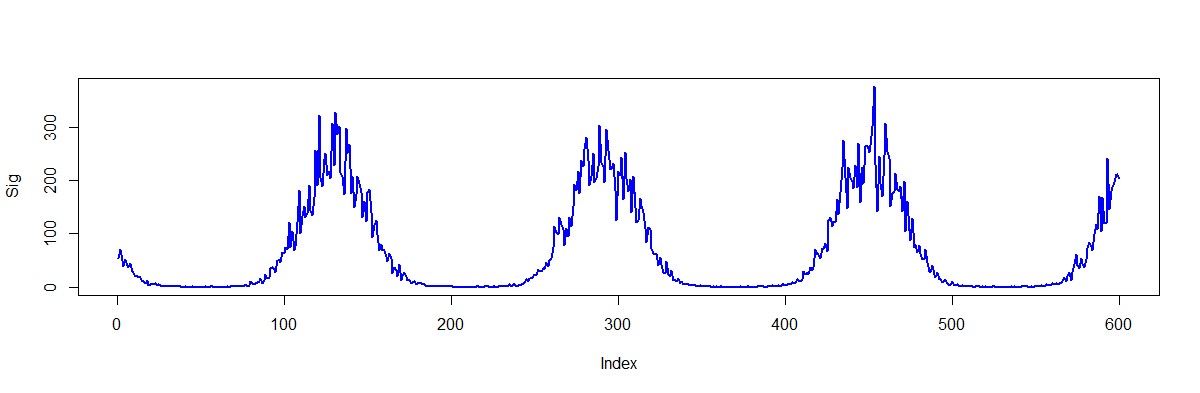
Fig. 3.  Metric representation example

However, it’s not difficult to see that the measured value lies within certain discrete ranges, the sequence of which can be traced over time. Thanks to quantization, this fact facilitates shifting from a continuous representation to a discrete one. Limit the number of measured values by a finite set breaking the entire values range to the equal density areas:

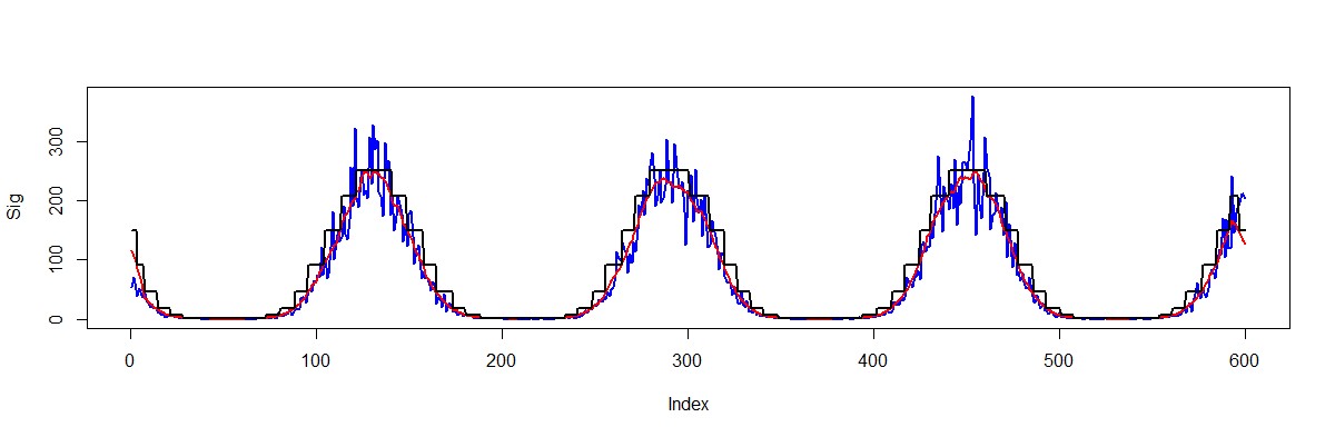
Fig. 4. Signal discretization

Taking the time factor (T) into account, it becomes possible to allocate those discrete random variable values that are highly unlikely for a specific time line. So, in our example, the beginning and end of the working day are characterised by discrete random variable values from the set {6, 18, 46}, while the range from 12:00 to 18:00 is characterised by a greater load. Here’s the correlation we get:

With this approach, the discrete random variable value (the analysed parameter) defined by a small occurrence possibility within any time axis area (time slot) means getting out of the overall pattern, and consequently – the anomaly. Thus, for the time interval from 9:00 to 12:00 we get:

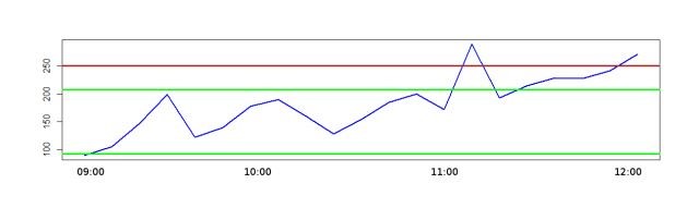
Fig 5. Possible value boundaries

Such interpretation makes it possible to simultaneously analyse measured parameter values for different categories; according to experimental data it may be established that the value of one category suits for adjusting metric values for the other . This means that there are common combinations of values in both categories. In this case, the information enhances certain pattern value. The more categories a frequent combination combines, the higher the detecting pattern probability in the observed process is, and the higher the deviation from it appears.

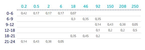
Let’s say, as based on the results of observations within one month, the following activity was recorded in two different settings (M1 and M2):

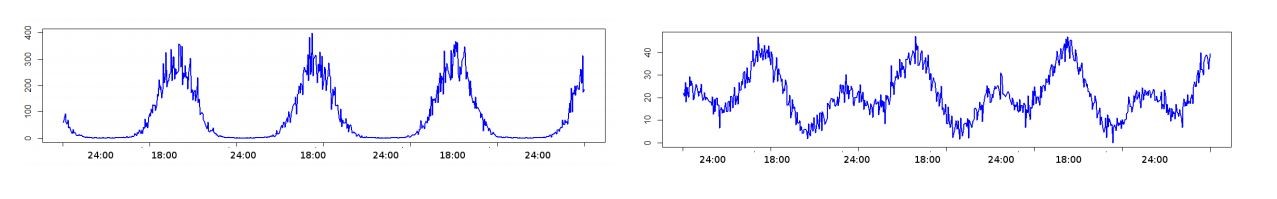
Fig 6. Observation results for two metrics

Dependence between individual values of the observed value can be represented as a graph, where nodes are random events (system’s state). Each event corresponds to a certain metric value or combination of several values, and link weights reflect their conditional probabilities (Fig. 7-left). As seen in the graph, the system behaviour is described by a pattern set that can be found in each observation (system’s state). This graph can be simplified by means of small weight connection levelling and path reduction with a low total weight (Fig. 7-right). As a result, we get a set of rules that define normal system behaviour.

The problem of obtaining user activity patterns in the network faces the problem of detecting associative links between individual states of the system described above, which form associative rules that describe the required patterns. This approach makes it possible to use known methods of mining association rules in order to recreate the average user activity, in particular the Apriory algorithm.

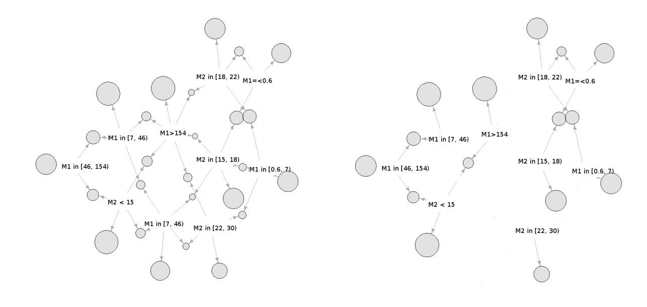
Fig. 7. Stochastic Model

Each of the rules selected is a component of the required user behaviour pattern: the bigger the number of rules for observation gets, the more significant the pattern may be considered, and the more likely it will characterise the expected behaviour standard. As the observation rank, we used a normalised meaning of the weighted rules. So for this example, we get:

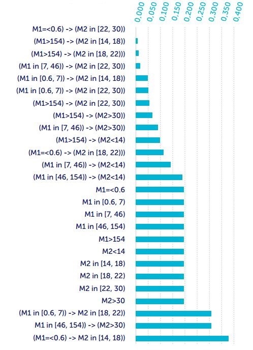
Fig. 8.  Rules importance

The lower the observation rank, the more reasons there are to believe that it is covered by the definition of anomaly.

The developed model allows several factors to be taken into account in assessing user activity, as well as describing it as a finite rules set, each of which is characterised by a certain level of significance in the found patterns system. Similar to the previous model, it can be used to analyse the process online, and adapted to the changing process due to the revaluation of the detected rules weight and/or by means of adding new ones.

Time Series Clustering

The last model is based on the time series partition method which allows a set to be presented as a discrete segments ensemble that forms separated groups (clusters) defined by the fact that time series components from the same cluster are close to each other, while the fragments from different clusters are distinct. Here’s an example of time series analysis:

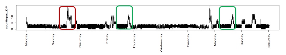
Fig 9.  Time series fragments similarity

Line fragments highlighted in green have more in common than a red-contoured one. In this case, they may be referenced to one group. To estimate the time series proximity degree (similarity), it is possible to use a timeline dynamic transformation algorithm (DTW) which facilitates the finding of optimal conformance by using time series fragments. This method was used in speech recognition. The process of time series segmentation presupposes formation of fragments plurality from this line by passing it with a floating window of a given size and with a certain sampling interval.

In general terms, Fig. 10 depicts the basic process of the model in question, i.e. detection of the time series abnormal dynamics.

The result of the pairwise comparison of the obtained fragments through a DW-distance evaluation forms the adjacency matrix which reflects the proximity degree between the fragments. The obtained matrix may be used as a basis for solving the issue of fragments clusterization.

The clusterization result of the first 13,000 minutes (80%) for three metrics (countInputUDP, countInputTCP and averagePacketSizeOutputUDP) is shown in the figure below. Fragments of the time series are displayed in the space of two principal components, while different colors distinguish components from different clusters. In each case a single large cluster is formed out of the time series fragments that constitute a common behaviour pattern. Clusters of small size can be interpreted as an anomaly.

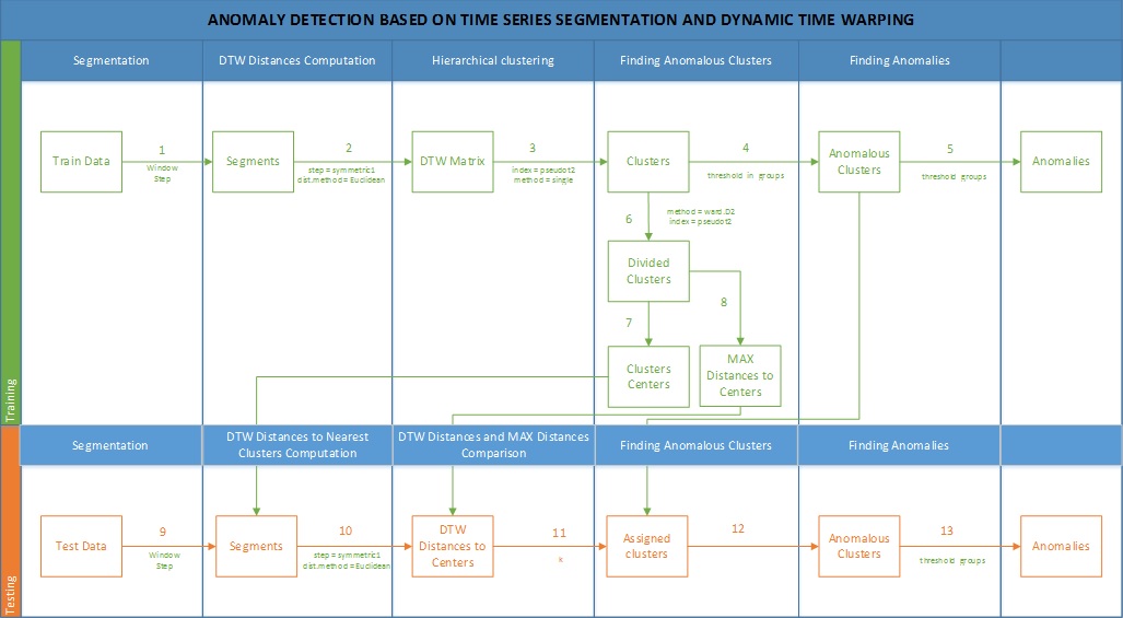
Fig 10.  Abnormal dynamics detecting process

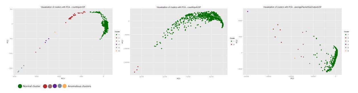
Fig 11.  Clusters representation

Clusters with small amounts of components are related to dynamics changes, which isn’t typical for the majority of cases. The level of these deviations abnormality depends on a relevant set power. At the same time, the significance of anomaly in a certain period of time can be determined by the number of metrics that were analysed to identify the period.

The obtained model allows network activity to be estimated through the dynamics of the measured parameter changes and/or measured parameters system, which may help identify abnormality even if the absolute values lie within acceptable ranges. The only drawback it poses is the complexity of usage “on the fly” because its implementation requires calculation of the similarity degree of the new observations with the existing clusters elements.

The next and the last part of this series will describe how the three suggested approaches work when combined.