Visualising Data at Scale with Ubuntu 14.04, Apache Spark and iPython notebook
 Richard Conway, Co-founder, Elastacloud and the UK Microsoft Azure Users Group
Azure has opened up a wealth of possibilities for startups and smaller companies that may have initially struggled with building large scale out technologies. As such, the cloud has become the home of the “transient cluster” which allows customers to spin up a large quantity of compute resource, process some data and spin the cluster down, thus only paying for what you use.
This article is about how you can meet scale out Big Data challenges using a Linux backbone on Azure.
Using Apache Spark
This is the first in a series of articles on building open source application patterns for scale out challenges. It will challenge the orthodoxy and offer alternatives to the Microsoft SQL stack and hopefully show you, the reader, how mature Linux on Azure is.
All examples are built on top of our customisable Big Data platform, Brisk. Brisk supports out of the box clusters of Apache Spark, Apache Kafka and InfluxDb that can be wired together in VNETs using complex topologies as well custom access to Azure Storage, Service Bus and the EventHub.
In order to “spin up” an Apache Spark cluster set yourself up an account on Brisk. For this you’ll need a live id and a valid Azure subscription. We’ll manage all the rest for you and your first cluster is free.
Apache Spark allows you to query large in-memory datasets using combinations of SQL, Scala and Python. For the purposes of this article we’ll focus on using python to visualise our data but in others in the series we’ll consider both Scala, Java and SQL.
Once you’re set up with Brisk which will entail that you upload a “publishsettings file”, which will allow us to deploy Apache Spark in your subscription, you can follow the wizard steps to create a cluster.
To setup your publish settings see here:
And then you can go through the Apache Spark cluster creation process here:
When the cluster is running you can download the .pem file which will give you SSH access to the cluster. We’ll need this to proceed so click on the download button as peer the image.
Once you’ve done this you should be able to SSH into the cluster using this username, password and certificate.
Depending on whether you’re using a mac or Windows machine you’ll use SSH in different ways. Mac users can add the downloaded file to their keychain and then use ssh from the terminal prompt. Windows users can download a great graphical tool called bitvise and load the key into the key table.
By default the Spark master can be accessed through <clustername> .cloudapp.net on port 22 where clustername is the cluster name you selected during the cluster setup steps earlier.
When we’ve SSH’d into the cluster we can enter the following command to start iPython notebook.
startipython.sh
This will then start the iPython notebook server and bind this to Apache Spark. In this instance we’re going to use iPython notebook to visualize data that we’ll be processing across several Spark cluster nodes.
2015-02-08 14:36:24.839 [NotebookApp] Using existing profile dir: u'/home/azurec
oder/.ipython/profile_default'
2015-02-08 14:36:24.842 [NotebookApp] WARNING | base_project_url is deprecated,
use base_url
2015-02-08 14:36:24.851 [NotebookApp] Using MathJax from CDN: https://cdn.mathja
x.org/mathjax/latest/MathJax.js
2015-02-08 14:36:24.872 [NotebookApp] Serving notebooks from local directory: /h
ome/azurecoder
2015-02-08 14:36:24.872 [NotebookApp] 0 active kernels
2015-02-08 14:36:24.872 [NotebookApp] The IPython Notebook is running at: http:/
/sparktest123.cloudapp.net:8888/ipython/
2015-02-08 14:36:24.873 [NotebookApp] Use Control-C to stop this server and shut
down all kernels (twice to skip confirmation).
The iPython notebook application is now available on https://<clustername>.cloudapp.net:8888/ipython through the web. If you haven’t used Python before, don’t worry, you’ll love it. It’s great for slicing and dicing data and doesn’t have the steep learning curve that other programming languages have.
After navigating to the web page we should see the following:
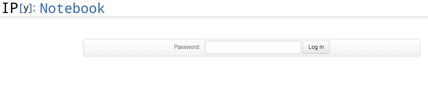
At the prompt you should enter the password you used earlier when you created the cluster.
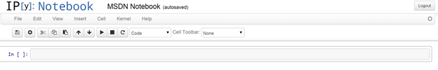
On the right-hand side we’ll click on the new notebook button to create a new iPython notebook. This will open a new webpage.
By default the notebook is called Untitled0 but if we click on the notebook name it will pop up a dialogue. In this instance I’ve changed the name to MSDN notebook.
One of the key features of Python is its ability to easily transform into something visible. This is because of the sheer number of available libraries. We’ll be using the matplotlib library to do this as well as numpyto access some maths functions.
import matplotlib.pyplot as plt
import numpy as np
To execute these commands from now on we’ll just hit the triangle button.
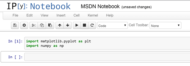
Now press execute.
For this article we’ll consider a simple dataset called AirPassengers.csv containing air passenger numbers between 1949 and 1960. There is more than one entry for each year so we’ll have to combine and average numbers for each year.
Copy this data from https://elastastorage.blob.core.windows.net/data/AirPassengers.csv and copy up to the default container you selected through the cluster wizard steps.
Enter the following:
Import re
lcsbasic = sc.textFile("/AirPassengers.csv")
withheader = lcsbasic.map(lambda line: re.split(‘,’', line))
withheader.count()
The output is arrays of Unicode strings including a header and should give us a count of 145 lines. Let’s get rid of the header now.
lcs = withheader.zipWithIndex().filter(lambda line: line[1] >= 1).map(lambda line: line[0]).persist()
The above is fairly interesting. We use the zipWithIndex function to pass an additional index value after every line and then discard the first index 0 which is the header row. We map back everything other than the index and the header row and then call persist() function which tell Apache Spark to store this filtered version of the datast in memory as an RDD (Resilient Distributed Dataset).
Running lcs.count() should reveal a count value of 144 now.
We can look at the first row with the following:
lcs.first()
Which should return us something like this:
[u'1', u'1949', u'112']
For now we can simply get the second and third values in the row and discard the first.
import math
mappedvalues = lcs.map(lambda line: (math.trunc(float(line[1])),math.trunc(float(line[2]))))
Now that we have our values mapped correctly to floats and truncated we can then build a Map Reduce function which will enable us to average all of the values over the years we’re looking at.
sumCount = mappedvalues.combineByKey((lambda x: (x, 1)),
(lambda x, y: (x[0] + y, x[1] + 1)),
(lambda x, y: (x[0] + y[0], x[1] + y[1])))
averageByKey = sumCount.map(lambda (label, (value_sum, count)): (label, value_sum / count))
sorted = averageByKey.sortByKey()
This is quite a lot to take in but what we’re doing is quite simple. The mapped values are being combined by the key values to give us a sum and count over the year. We can take this and use both these values in a second map function to calculate the mean values by year. Sometimes shuffling between nodes can skew the order so we can then perform a sort on the keys.
yearseries = sorted.map(lambda (key, value): int(key))
passengerseries = sorted.map(lambda (key, value): int(value))
The return value will now be perfect to fit back as some sort of plot so that we can determine the moving average over years.
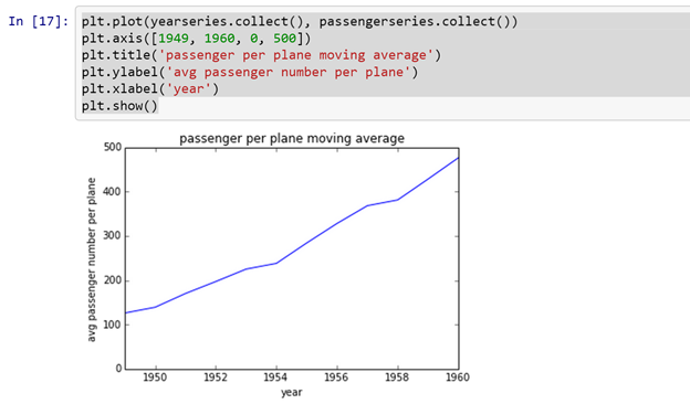
plt.plot(yearseries.collect(), passengerseries.collect())
plt.axis([1949, 1960, 0, 500])
plt.title('passenger per plane moving average')
plt.ylabel('avg passenger number per plane')
plt.xlabel('year')
plt.show()
If we look at the graph it produces you can see that we get a nice pattern of climbing passenger numbers per plane as the years advance.
In this post we’ve looked at how we can use an Apache Spark cluster through Brisk and easily give visualization to data by leveraging the power of scale out over Linux nodes on Azure. Brisk has also enabled us not to know about the internals of Spark.
In the next post we’ll look at how we can leverage large datasets with Apache Spark and how to use in combination with InfluxDb, a new open-source time-series database.