How To: Show pivot table data in flat format
As a seasoned Excel user, you are no doubt familiar with Pivot Tables and how they work. (If not, here's a great place to get started on them: https://office.microsoft.com/en-us/excel-help/pivottable-reports-101-HA001034632.aspx). Perhaps you've wanted to see your pivot table data differently. We know how to pivot the tables to display our data as needed, but what if we need to see all of the data for a field in a single flat format? How can we do this?
Consider the following sample pivot table:
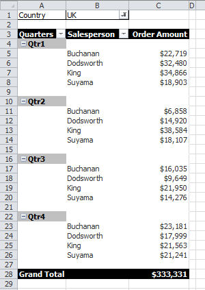
In order to show the data in flat file format, we need to be showing Grand Totals as we are with this table. If you aren't seeing grand totals, right click in your pivot table, left click PivotTable options. Click the 'Totals & Filters' tab and make sure both 'Show grand totals for rows' and 'Show grand totals for columns' are checked.
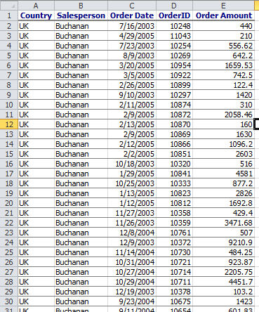
To display the data in a flat format, just double click the Grand total. What you get is the flat data (like the sample below) on a new tab added to your workbook.