Hidden Gems #11: Conditional Formatting

In this edition of Hidden Gems, we discover one of the most powerful aspects of Microsoft Excel: Conditional Formatting. With data so readily available, it’s easy to lose yourself in numbers and never see the bigger picture.
Instead of business decisions being a complete mystery, it would be helpful if the clues to actionable knowledge were more apparent. It would be even better if those clues simply made themselves known of their own accord. That’s exactly what Conditional Formatting achieves.
Case Notes...
The Target: Microsoft Excel, all editions from 2001 onwards, with refinements since then adding progressively more functionality.
Whereabouts: Included in all editions of Microsoft Office 2010. Trial version, training and lots of free templates also available.
Modus Operandi: Uncover trends and display key information in complex datasets intuitively and naturally – so that everyone can understand what they see.
Appearance:
Case History...
Finding raw data isn’t a problem – you’ve probably got lots of it. All those invoices, lists of customers and transactions, parts numbers or stocks lists are the sorts of data which businesses are made of. But with long lists of data, digging out the useful stuff from which to make worthwhile business decisions can be much harder.
The answer is Conditional Formatting; which in layman’s terms means changing the appearance of spreadsheet cells according to what you find in them. This means you can highlight important information, spot trends, or simply make information easier for you or the people you work with to understand.
Highlight Values
To illustrate the point, we’re going to bring back a spreadsheet of customers which last appeared in Hidden Gems six months or so ago. Only, this time, we’re giving it a makeover.
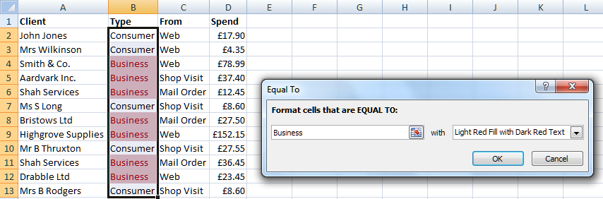
In the “Type” column, let’s highlight customers who are businesses rather than individuals.
Select the cells which are to be tested. On the Home tab, hit Conditional Formatting. Select Highlight Cells Rules. In this case, we’re looking to highlight cells that are equal to “Business”; and we’ll go for one of the several very reasonable pre-set highlights; in this case a light red fill with dark red text. As you can see, this neatly highlights the records which contain businesses.
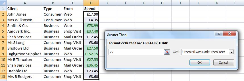
Similarly, let’s show which customers have spent more than £25 (Highlight Cells Rules > Greater Than > 25)
We can also automatically highlight records in the column which fulfil relative criteria; for example:
- The top or bottom X of the list (e.g. the top three)
- The top or bottom X% of the list (e.g. the bottom 20%)
- Above or below average values in the list
For these functions, select Conditional Formatting > Top/Bottom Rules.
Highlight based on data
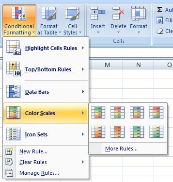
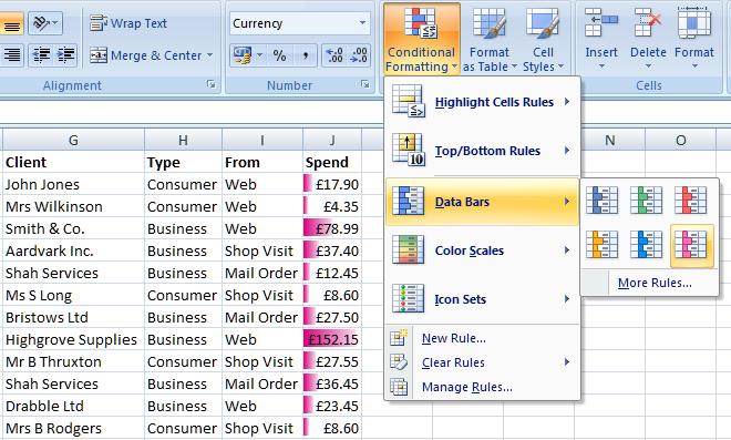
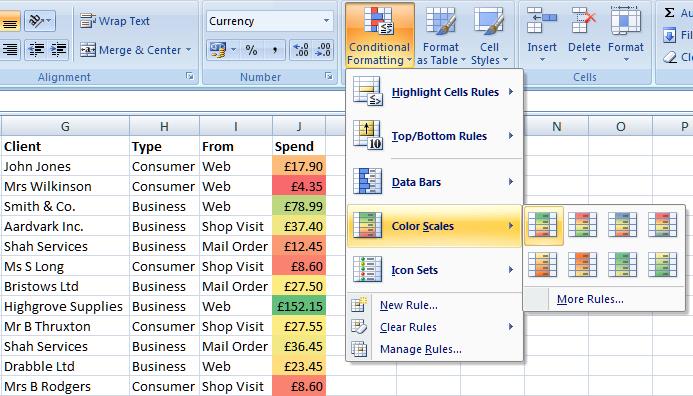
To make numeric data easier to understand, you can format numeric cells with a range of intuitive visual formats with only a couple of clicks. Hit Conditional Formatting > Data Bars and select a colour to have the cells in the range coloured in bar-chart style, automatically scaled between the lowest and highest values.
Colour Scales (Conditional Formatting > Colour Scales) operate in largely the same way; using two or three colour blends to chart progress across the data range. This makes it particularly easy to create RAGlists (Red – Amber – Green) identifying priority issues or transactions which need your attention. In our example below, we can easily see which are the low-value transactions (red) which might make less business sense.
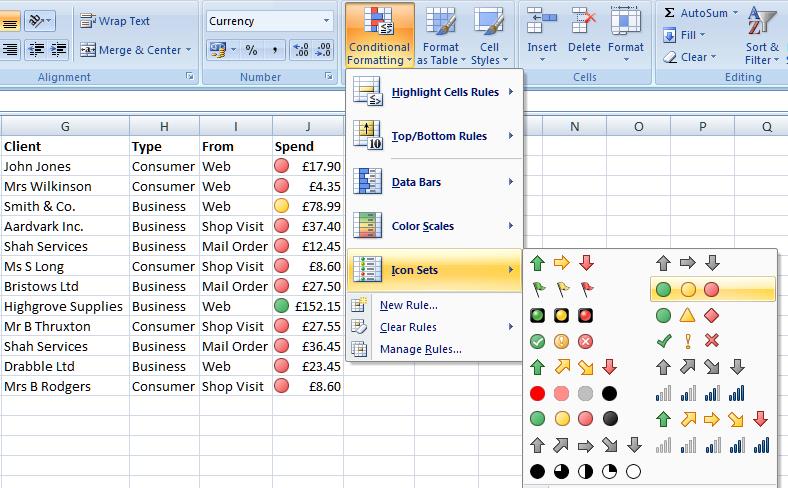
Indeed, hit Conditional Formatting > Icon Sets to find RAGList traffic lights and a range of other arrows, flags and scales for further intuitive demarcation of values, as shown below. Note, though, that Data Bars are visually most usefully accurate. The Icon Sets view below would suggest that all but two of our transactions are dangerously low-budget; yet that may simply be a case of my company stocking mainly low-value items. Since icons and graphics are going to influence the way a spreadsheet is interpreted, it’s important to pick the right motifs for the job.
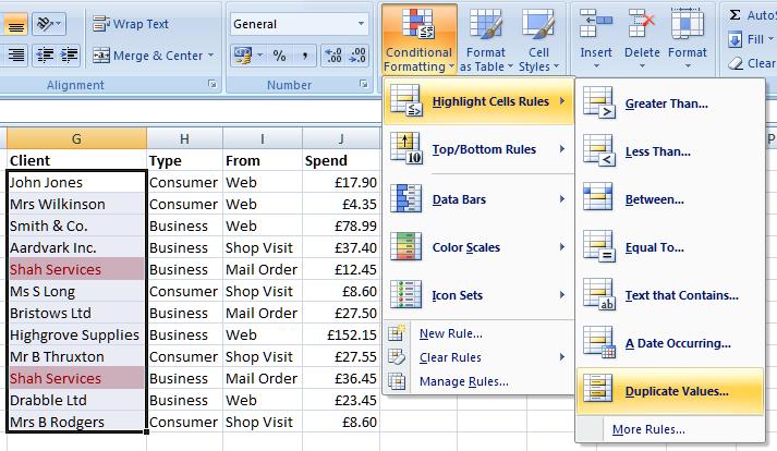
There is one more very useful shortcut to mention, namely the automatic identification of records with duplicates. Select Conditional Formatting > Highlight Cells Rules > Duplicate Values to have records identified which contain the same value. In our example, we have highlighted the first column, in which clients’ names are listed. By highlighting duplicates, we can see which clients have come back more than once:
Under the magnifying glass...
For the most customisable (but equally therefore more complicated) definitions of conditional formatting rules, select Conditional Formatting > New Rule and define one by hand. With this tool, you can:
- Change the colour schemes used to highlight data
- Mix numbers, percentages and relative values as the start and end points of conditional formatting validity
- Use formulae (which can even refer to additional data points) to define the application of formats
- Test for dates, blank cells or errors as well as numeric values
The target exposed
Find out more: