Analyzing Storage Performance using the Windows Performance Analysis ToolKit (WPT)
Introduction
Performance problems, especially as they may relate to the storage subsystem, can be quite difficult to troubleshoot. Enterprise storage technology has come a long way since the SCSI controller with an array of disks. Fortunately, there are some great tools available to help narrow down where to look more closely for storage performance problems. This blog post covers the Windows Performance Analysis Toolkit (WPT), as used for analyzing performance in the storage subsystem.
The facility that enables the analysis I am about to cover is called "Event Tracing for Windows" (ETW). The Performance Analyzer is built on top of the ETW infrastructure. ETW enables Windows and applications to efficiently generate events, which can be enabled and disabled at any time without requiring system or process restarts. ETW collects requested kernel events and saves them to one or more files referred to as "trace files" or "traces." These kernel events provide extensive details about the operation of the system. Some of the most important and useful kernel events available for capture and analysis are context switches, interrupts, deferred procedure calls, process and thread creation and destruction, disk I/Os, hard faults, processor P-State transitions, and registry operations, though there are many others.
One of the great features of ETW, supported in WPT, is the support of symbol decoding, sample profiling, and capture of call stacks on kernel events. These features provide very rich and detailed views into the system operation. WPT also supports automated performance analysis. Specifically, xperf is designed for scripting from the command line and can be employed in automated performance gating infrastructures (it is the core of Windows PerfGates). xperf can also dump the trace data to an ANSI text file, which allows you to write your own trace processing tools that can look for performance problems and regressions from previous tests.
The following information will be mostly about the WPT tool called "Xperf.exe". Xperf.exe is the command line tool used to start, stop, and manage traces. The usage of Xperf.exe is documented thoroughly in the help file included with the WPT titled "WindowsPerformanceToolkit.chm".
Obtaining the WPT Tools
The WPT comes with the Windows Software Development Kit (SDK), which is a free download
Microsoft Windows SDK for Windows 7 and .NET Framework 4
https://www.microsoft.com/download/en/details.aspx?displaylang=en&id=8279
You can install just the WPT from the SDK using the custom installation option. You can also choose to just download the WPT as a Windows Installer file (.MSI) in case you need to install that later on other machines. The .MSI packages are delivered under the section called "Redistributable" components. There will be 3 .MSI files, one per machine type architecture (x64, IA64, and x86).
One important thing to note about the WPT. You can capture a trace from a running production computer without making any changes to that computer. That is, you do not need to install the SDK, nor the .MSI package. You can install the WPT on a different machine, even a virtual machine. Then you can just copy the files, folder, and sub-folders to the production machine. In fact, you really don't need to copy all the files to the production machine, just the analysis machine. The following blog has documented that you need just two application files; Xperf.exe and Perfctrl.dll:
Xperf Articles:
https://blogs.msdn.com/b/pigscanfly/archive/2008/03/15/xperf-articles.aspx
More About the WPT
Windows Performance Analysis Tools
https://msdn.microsoft.com/en-us/performance/cc825801.aspx
WPT and XPerf utilize Event Tracing for Windows to record system activity that can later be used for performance analysis. Here is more about Event Tracing for Windows:
About Event Tracing
https://msdn.microsoft.com/en-us/windows/hardware/gg487334
CL16: Performance Analysis Using the Windows Performance Toolkit
https://ecn.channel9.msdn.com/o9/pdc09/ppt/CL16.pptx
In fact, the blog above has great information about getting started. The only other real "best practice" would be to use the same version of Xperf for the respective architecture (x64 for x64, x86 for 32-bit, IA-64 for Itanium).
Getting Started: Capturing Storage Performance Data
Scenarios
Here are scenarios that you would use the WPT:
- Start the trace from a batch file, based on anticipated load. For example, the storage seems sluggish at a particular time, so a trace is started at that time, run for some period of time, and then stopped.
- Run a trace in "circular mode", which means the trace runs all the time, but is limited to a pre-determined size. The pre-determined size might be 1 GB, which on most system allows a good time "window", though the size is impossible to predict. 1 GB might be 30 minutes on 1 system or 10 on another, depending on number of Logical Units (LUs), workload, etc. And, you can certainly make the trace larger, just keep in mind the analysis machine and the time it takes to load and process the resulting trace file.
Considerations for Starting a Trace
Once you get the files copied to the target server, or the WPT installed, you can start a trace easily by going to an "administrator" .CMD prompt and running:
|
If you run that command and get no feedback, you are capturing a trace. You will only get feedback if there is an error or if a "kernel" trace is already running, as is the case with the following example:
|
From this point, the trace captures to buffers in memory and periodically flushes the trace information to a disk file. One thing to keep in mind is that the Xperf process does have a small amount of overhead of RAM for buffers, CPU for processing the trace events, and storage performance and space for the target disk device. The output from Xperf can be directed to a particular location. Generally you are safe to start your trace in the same volume as your operating system is installed, or some other volume other than the one being analyzed. You can start your trace on a different drive, or use the "-f <location>" parameter to redirect the WPT output.
NOTE: There are many different components that you can trace using Xperf. For storage performance analysis, here are some suggested ways to start Xperf, along with the charts available in the resulting traces:
xperf -on FileIO+Latency+DISK_IO+DISK_IO_INIT+SPLIT_IO
Xperf -on FileIO+DISK_IO+DISK_IO_INIT+SPLIT_IO
The differences in the above commands are the result of parameters passed in to Xperf when starting a trace. There are many different parameters that can be used to start a trace. The parameter above, “diag”, is a group (kernel group) of commonly used parameters. Here is the list of kernel groups available with the 7.1 WPT version of Xperf:
Kernel Groups:
Base : PROC_THREAD+LOADER+DISK_IO+HARD_FAULTS+PROFILE+MEMINFO
Diag : PROC_THREAD+LOADER+DISK_IO+HARD_FAULTS+DPC+INTERRUPT+CSWITCH+PERF_COUNTER+COMPACT_CSWITCH
DiagEasy : PROC_THREAD+LOADER+DISK_IO+HARD_FAULTS+DPC+INTERRUPT+CSWITCH+PERF_COUNTER
Latency : PROC_THREAD+LOADER+DISK_IO+HARD_FAULTS+DPC+INTERRUPT+CSWITCH+PROFILE
FileIO : PROC_THREAD+LOADER+DISK_IO+HARD_FAULTS+FILE_IO+FILE_IO_INIT
IOTrace : PROC_THREAD+LOADER+DISK_IO+HARD_FAULTS+CSWITCH
ResumeTrace : PROC_THREAD+LOADER+DISK_IO+HARD_FAULTS+PROFILE+POWER
SysProf : PROC_THREAD+LOADER+PROFILE
Network : PROC_THREAD+LOADER+NETWORKTRACE
The main advantage of gathering one set of parameters versus another is that you have more information to drill down into by adding the “latency” kernel group flag. The down-side will be larger overall trace size, and a bit more overhead on the system being measured as the traces are running.
Stopping a Trace
When you are ready to stop a trace, you can easily stop with the "-stop" parameter of Xperf.exe. In nearly all cases however, I would recommend using the " -d" parameter to stop (and merge) a trace. The only time you wouldn't be concerned would be if the trace and analysis computer were the same computer.
|
The difference between the two parameters is that "-stop" simply stops the capture and flushes everything to disk, while "-d" does the same but merges additional information about the current system into that trace. The benefit of using "-d" is that the trace is now portable, meaning you can copy that to a different machine and perform analysis there. This is what happens most of the time with production systems, because we usually don't want to be analyzing traces on servers that are busy doing production work.
One consideration when stopping a trace is the file name. You will probably want to keep the suffix the same (.ETL), but you may want to name the trace file to include the computer name, date, time, or other aspects of the trace. This just helps later if you have multiple trace files to manage from multiple systems.
Another consideration is identifiable information in the trace. When traces are taken, items are recorded such as computer names, file names, paths, etc. This is just an additional consideration. One way to get the recorded data and scrub out private information is to export to a file from the trace, and then filter or delete from your second analysis tool, such as Excel. There are other ways to accomplish the data scrub if needed, such as PowerShell scripts, LogParser, etc.
Trace Analysis
There are two different ways to initiate trace analysis with the WPT; command line or GUI. With the GUI tool, you can start the trace viewer by running "Xperfview.exe" from the Start menu, then from the tool called "Windows Performance Analyzer", click File, then click Open, and then browse to the trace file being analyzed. If you prefer the command line, run "Xperf <filename.etl>". If you run Xperf from an "administrator" level .CMD prompt, you will get the following message pop-up:
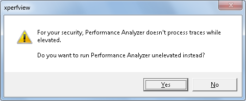
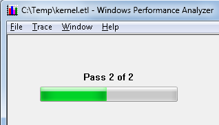
Clicking Yes will allow the trace processing to continue, clicking No will terminate the trace processing at that point. Once the trace begins to load in the trace tool, you will see activity as the trace processing moves through it's phases:

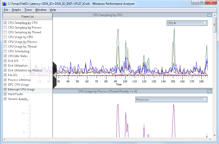
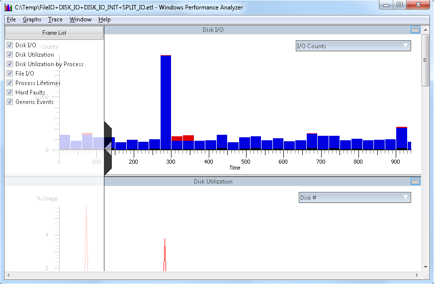
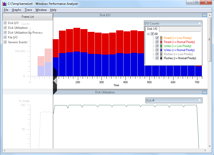
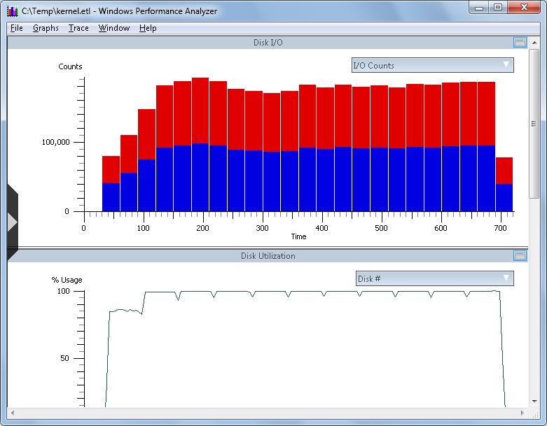
Once the trace is fully loaded, you will see the trace depicted graphically in the Xperfview tool. For storage performance analysis, you can get down to I/O by starting at the "Disk I/O" chart, as shown below in a sample trace:

From the screen capture above, and in the DIsk I/O chart context, you have the following elements:
- X-Axis: This is the horizontal "time" line, which is from the time the trace initiated until the trace capture stopped (in seconds)
- Y-Axis: The value of the vertical Y-axis will change depending on this chart you are viewing. In the first example above, you can see I/O counts.
- Top-Right "flyout": (downward pointing arrow to the right in the bar labeled "IO Counts") Changes with chart. In the top example, this is I/O Counts with red being read I/O and the blue being write I/O
Clicking once will open the flyout, clicking again will close the flyout. - Left middle "flyout": (right pointing arrow midway up the left side of the chart) This is the "Frame List", and allows you to select or deselect charts for immediate viewing in the Xperfview tool.
Clicking once will open the flyout, clicking again will close the flyout.
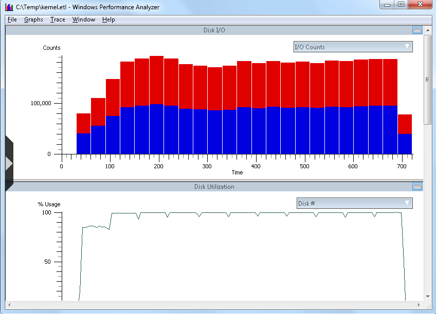
Here is the same chart as shown above, with both flyouts open:
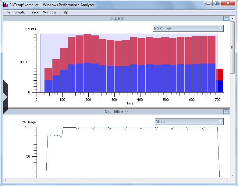
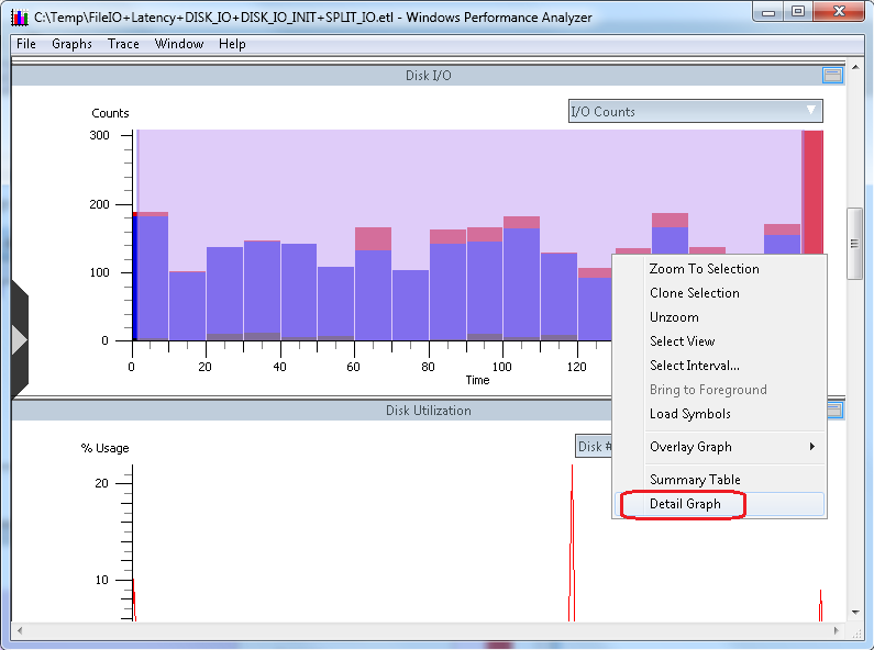
At this point, we will drill down into the data. Point your mouse cursor to a section of the top-most chart, left-click and hold, and then swipe the mouse right to select an area to drill down into. Your selection may look something like this:
Now, point the mouse cursor to any part of the shaded area of the "Disk I/O" chart, right-click, and you will have a context menu pop-up with additional actions available:
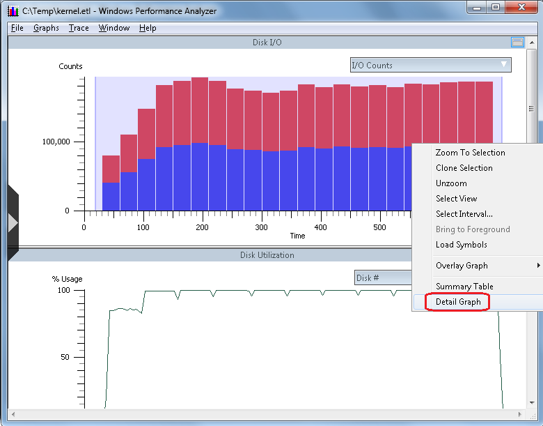
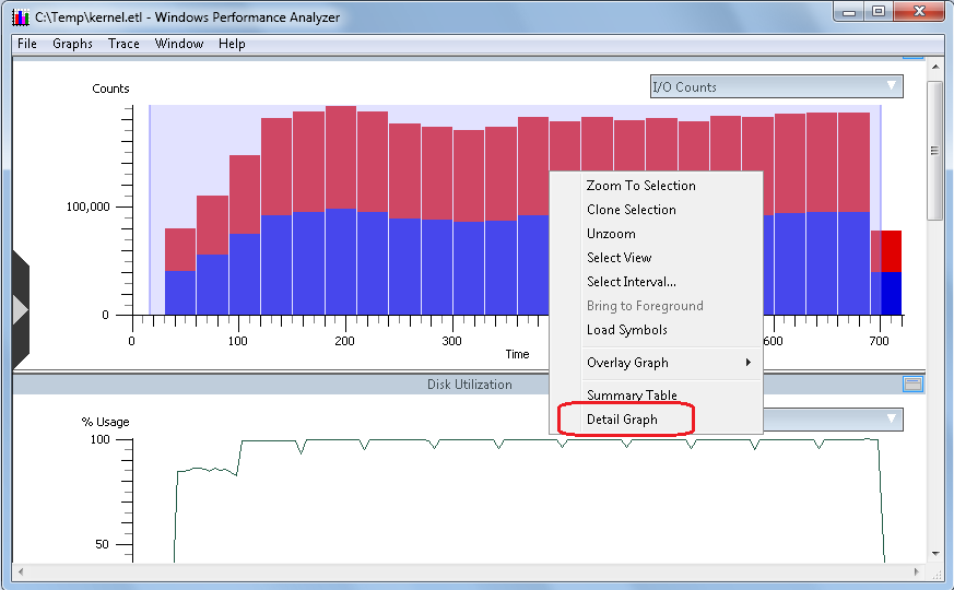

For our purposes, point to the option called "Detail Graph", and then left-click Detail Graph to open a new chart that looks like the following:
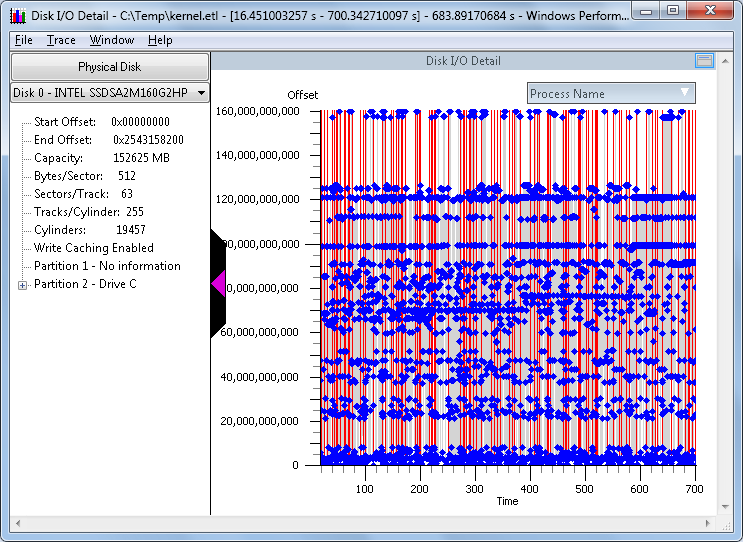
This new chart is called the "Disk I/O Detail" chart. The first thing that stands out is the visual representation of the I/O on the disk during this trace sample. For example, you can quickly spot trends such as sequential I/O, random I/O, or concurrent I/O with mixed workloads such as sequential and random at the same time on the same disk
The various elements of this chart are as follows:
- Detail about the disk on the left pane
- Left-upper pane drop-down, under the section called "Physical Disk". This allows you to change the view to a different physical disk
- Upper-right side flyout titled "Process Name". Clicking this allows you to select and deselect I/O from various process that were running at the time the trace was captured.
- X-Axis (time): This is the time, in seconds, of the area previously selected when we swiped to select an area of the previous chart for analysis.
- Y-Axis (Offset): This is the offset from the beginning of the physical disk, to the end of the physical disk.
NOTE: The Offset value next to the color-chart is decimal, and the Offset value in the information pane on the left side is in hexadecimal.
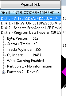
Next, choose the "Physical Disk" that you would like to analyze. in the example above, there is a "Disk 0 - Intel...". Next to that you will see a down-arrow. Click the down-arrow and you can click to view a different physical disk:
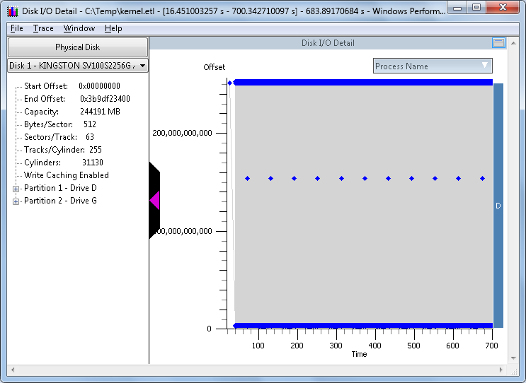
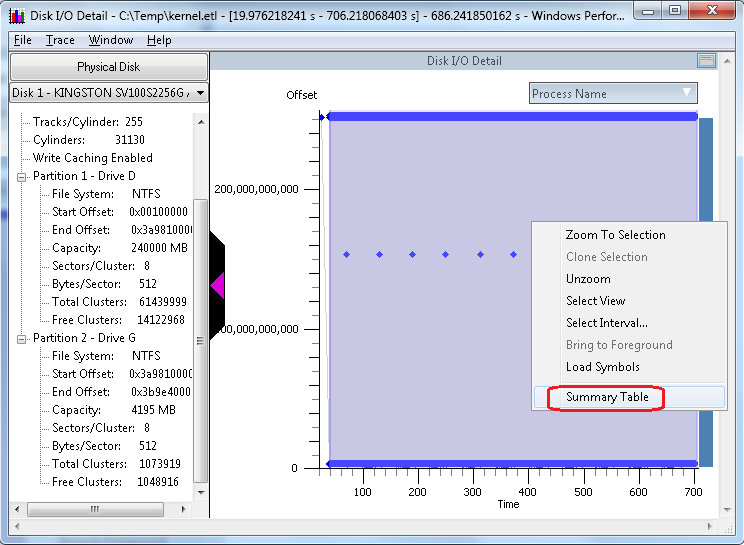
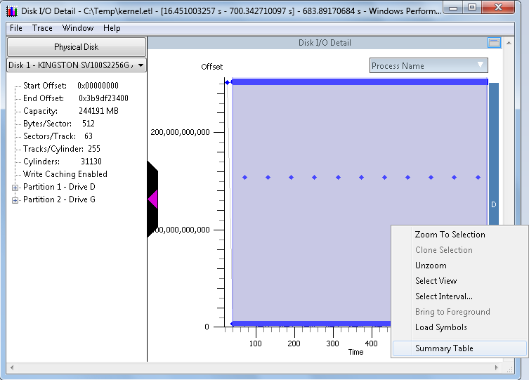
From here, clicking a different disk, such as "Disk 1", will change the chart to reflect the new disk selection. You will get information about the disk, as well as the partitions on the disk. The graphical view is a depiction of the disk and the I/O that occurred during the sample interval, with time going left to right and location of I/O on the disk going bottom to top. In this example, the trace interval was 700 seconds, and there were 2 concurrent workloads to relatively small files, concurrently. There was one file on a partition with drive letter "D", and another file on a second partition with drive letter "G". For a concurrent workload like that, you would normally expect there to be some penalty involved with disk seek, as would be the case with rotational disk drives. But this test was performed using a Solid-State Drive (SSD), so there is no seek penalty.
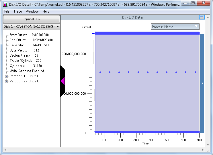
Now, point to an area of the chart above, somewhere towards the left side of the graph, left-click, hold, and swipe right to highlight a section of this graph to analyze further. Your selection may look something like this:
The next image depicts Xperf with the partition information expanded (click the plus-sign next to partition to expand) and the "right-click" context menu.with "Summary Table" highlighted:
On the context menu, click the option called "Summary Table" to open a new window, which is a detail view of the I/O that took place during the interval of the sample selection. Your chart might look like this:
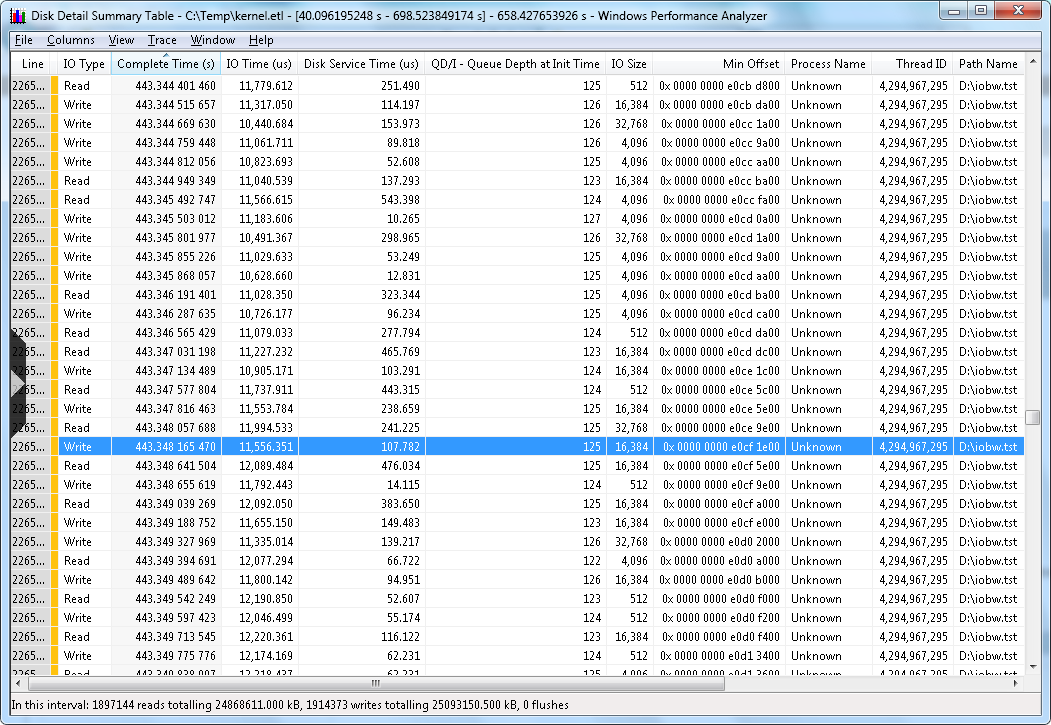
This is a table, that is the result of every I/O from the sample that we drilled down into from step 1. Recall that the first step we chose maybe all, or maybe part of that first chart. Then in the second step we once again had a choice to select the entire chart, or only a portion. This table contains a wealth of information about the I/O that occurred during the trace collection.
The elements of this table are as follows:
- Each line represents a single I/O, numbered based on the number of I/O in this sample interval
- Each column contains information relevant to that I/O
- You can sort the table by the column of your choice. The sample above is sorted by "Complete Time", which will display the trace I/O top to bottom, via time of I/O completion. You could for example click the column header "QD/I", and then you could see what was going on at various points with respect to I/O queueing.
| Line | Line number of the individual I/O |
| IO Type | Read, Write, or Flush |
| Complete Time | (Milliseconds) Time of I/O completion, relative to start and stop of the current trace. (not clock time and not overall I/O completion time) |
| IO Time | (Microseconds) Amount of time the I/O took to complete, based on timestamps in the IRP header for creation and when the IRP is completed. These measurements come from the partition manager level in the Windows kernel. |
| Disk Service Time(micro-seconds) | (Microseconds) An inferred duration the I/O has spent on the device, based on several assumptions:- A single I/O in flight- No I/O delay if the disk is available- A single disk service time interval per I/O, tucked at the end of the I/O time interval, and- Disk service time of another I/O completionThe disk service time interval spans (backwards in time) from the completion of the I/O back to the latest preceding completion of some other I/O on the same physical disk or the initialization of the I/O, whichever is later. Disk service time is a valuable measurement but has limitations. There can be multiple I/O in flight, I/O issuing delays (low-priority I/O), I/O reordering below the partition manager, etc. |
| QD/IQueue Depth at Init | Queue depth for that disk, irrespective of partitions, at the time this I/O request initialized |
| IO Size(bytes) | Size of this I/O, in bytes. |
| Min Offset | Relative location of this I/O, from beginning of the disk, based on Logical Block Address (LBA) |
| Process Name | If known, the name of the process that owns the thread that initiated this I/O. Getting the process name depends on what flags you use when you start the trace. |
| Thread ID | Thread identification number. |
| Path | Path and file name, if known, that is the target of this I/O. |
What to Look For
Right away you get information on the bottom status bar of how many I/O are in this sample, and of those, how many are reads and how many are writes. There are other types of I/O, such as flushes that might be found in a trace. You can look at disk queuing and find out if queuing is impacting performance.
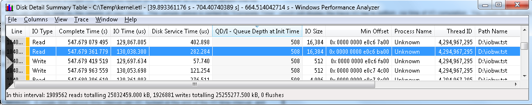
In this sample we see a read I/O that took around 130 ms to complete, which is not very good. We can see from the column QD/I that the disk queue length at this time was 508, and the inferred time spent waiting on hardware was .282 millisecond. On an SSD drive, .282 ms I/O time is pretty common. On a rotational drive, you would see similar response times at various points in your trace.. If you were viewing a trace from a rotational disk, and you see sub-millisecond response time, you can conclude that this I/O was serviced by cache at some point, either the cache directly on the disk, or cache on a storage controller somewhere. What we can conclude from this I/O was the slow response time was the result of too many I/O being sent at one time, perhaps from a multi-threaded application, You might see something like that from a stored procedure in a database application, a log checkpoint, or a simultaneous burst of I/O on an already busy disk.
At this point what you want to look for is the length of this event. We need to determine whether this was a short-lived event that we might possibly tolerate, or was this a sustained event that resulted in poor storage performance for a length of time. In the case above, I was running stress on a disk just to see how many I/O I could build up and you can see the result. At some point you will cross the threshold of poor performance by adding more and more concurrent I/O. This is one of the many great uses of this table view of all the I/O. I can line up the I/O based on response time, and then I can just determine how many of those I/O cross the boundary to poor I/O performance. Here is an example:
- Start by clicking the column header called 'IO Time (us)". This will sort the I/O by overall I/O completion time.
- Scroll down until you reach the threshold of performance from say "great" to good". This might be where we cross the line from under 10 ms to over 10 ms.
- Add up the total number of I/O
- Divide the line number of the threshold into the overall total number of I/O. For example:

Figure 12. Disk Detail Summary Table with I/O sorted by IO Time
In Figure 12 the areas to sort on are highlighted. Starting at the top and going counter-clockwise, I/O Time, Line Number, Total number of reads, total number of writes are all circled. Add reads and writes to get 3,840,592. Divide your total IO (3,840,592) by the line number (2,063,791) and the result is 0.537 (and change). From this we could conclude that 53.7% of our I/O in this sample completed in less than 10 ms. Or we could conclude that 46.3% of our I/O took more than 10 ms.
We then go back to our storage performance requirements. We might require that 90% of our I/O complete in less than 10 ms. The conclusion from this trace sample would then be that the storage subsystem does not meet our performance requirements based on the workload that the storage subsystem experienced during this trace sample.
What are We Doing Here?
Probably the first thing people want to know when troubleshooting storage performance is what to blame. Is it the storage? Is it the operating system? Is it the application? What performance measurement tools can help determine is where to start looking. If for example we see a high number of I/O that take more than 10 ms to complete outright, as evidenced by the "Disk Service Time" statistics, we can conclude what side of the Partition Manager (PartMgr) the problem resides. There are still a few Windows components left after PartMgr and before we hand off to the hardware. If we determine that I/O is building up (queuing), overall I/O completion time is high but disk service time is low, then we can look towards the operating system side for our efforts.
High Disk Service Times
There are numerous reasons why Disk Service Time numbers might be high:
- Direct-Attached Storage
- Storage subsystem is not keeping up with load
- Partition Misalignment for RAID disks
- Failing component in storage subsystem
- Storage Area Network (SAN)
- Sending too many I/O at one time
- Too many hosts per fabric port
- Too many hosts per storage port
- Failing component(s) in SAN fabric
Recommendations:
- Lighten load, or spread out load over time
- Add disk devices
- Ensure partitions are aligned (Microsoft KB 929491)
- Enable Storport tracing to confirm slow I/O below the Storport layer, which is the last layer of Microsoft software in the storage "stack" before passing the I/O to the hardware miniport driver. Storport hands I/O to the storage hardware driver, be that Fibre Channel miniport, Storport miniport (direct-attached), or iSCSI hardware driver. See the section below on Storport tracing.
- If SAN:
- Check statistics on fabric ports between this host and storage target. Look for:
- BUFFER_0 errors
Fibre Channel SAN switch ports use buffers to handle incoming and outgoing frames. There are a limited number of buffers per switch port. If a switch port runs out of buffers it will return a "BUFFER_0" error to sender and refuse I/O. As soon as a buffer is freed the port will return an idle frame indicating a free buffer. These errors are not returned up to OS, though they are visible to the host-bus adapter (HBA). By default, the HBA will probably not report or log an associated error, because these errors are presumed to be ephemeral in nature. There may be logging in the HBA that you can enable that will return BUFFER_0 errors. This extended logging will add overhead somewhere. - CRC errors
Indicated corruption within the frame - Enc errors
Indicates errors at the 8b/10b encoding level - Link Errors
- Loss of signal
- Loss of sync
- BUFFER_0 errors
- NOTE: The person troubleshooting doesn't necessarily have to understand what all the statistics means down to the specification, but just understand what is considered "normal" and what is not. Generally it is not normal to see a lot of CRC or ENC (encode) errors. This could indicate a hardware problem. The problem could be a SFP connector, it could be a bad fiber-optic cable. There have been cases where all the hardware checks out good, and the problem disappeared when changing the fiber-optic cable. In some cases a smudge on the end of the fiber cable was the root cause. There could also be dirt of debris on the inside of the SFP connector. These can be tough to track down, and sometimes require replacing hardware or a hardware analyzer trace to determine root cause.
- Check statistics on fabric ports between this host and storage target. Look for:
Storport Tracing (For Storport storage devices)
Storport.sys in the Windows storage port driver designed to handle IO requests for most storage devices on servers. PCs, laptops, and other computers that use SATA drives for example, or even SSD drives, probably are using the ATA port driver (Ataport.sys).
If the storage hardware in the server being measures uses a Storport driver, and is in some way suspected of poor performance, additional Storport tracing is available to report "slow" I/O. Storport ETW tracing has been available for a few years now. There is more information available on this topic in the following KB article:
A hotfix is available that improves the logging capabilities of the Storport.sys driver to troubleshoot poor performance issues for the disk I/O in Windows Server 2008
https://support.microsoft.com/kb/979764
NOTE: Microsoft hotfixes are cumulative. The tracing in hotfix 979764 is available in that fix, plus all subsequent fixes. And, that functionality would be rolled forward to any subsequent operating systems.
This additional tracing, which we would only want to enable during a troubleshooting session, will report I/O that took longer than xx ms to complete, as measured from the Storport level within the operating system. Storport.sys is the last layer of software in Windows that an IRP will pass through before being handed off to hardware, such as an HBA miniport driver. These events will be reported in the Windows event log. The ETW traces are great, but this is at a level lower than even the Xperf traces, so removes one or more layers in the storage "stack" as possible causes of I/O slowdown.
High IO Times
There are numerous reasons why IO Time numbers might be high:
- Single jobs or applications sending too many I/O in short bursts
- Concurrent jobs or applications sending too many I/O in short bursts
- "Filter" drivers stalling I/O (intentionally or unintentionally)
- Anti-virus
- Screening
- Quota
- Firewall
- Multi-Path I/O
- Windows "kernel" thrashing
- Trimming operations
- Cache operations
- File/Object contention
- Volume Shadow Copy operations
Conclusion
The Windows Performance Analyzer Toolkit is a powerful addition to your tool set for analyzing storage performance. The uses of WPT go far beyond storage, but when it comes to storage, provide an extremely valuable tool to take a very close look at what is going on with I/O on your systems.