How to Use FPGAs for Deep Learning Inference to Perform Land Cover Mapping on Terabytes of Aerial Images
This post is authored by Mary Wahl, Data Scientist; Daniel Hartl and Wilson Lee, Senior Software Engineers; Xiaoyong Zhu, Program Manager; Erika Menezes, Software Engineer; and Wee Hyong Tok, Principal Data Scientist Manager, at Microsoft.
AI for Earth puts Microsoft's cloud and AI tools in the hands of those working to solve global environmental challenges. Land cover mapping is one goal of the AI for Earth program, which was created to fundamentally change the way that society monitors, models, and ultimately manages Earth's natural resources. The ability to perform ultra-fast land cover mapping using deep neural networks on terabytes of high-resolution aerial images from the National Agriculture Imagery Program (NAIP), provided by our partners at Esri, fuels new intelligent AI applications, delivering quick insights to land cover map users like conservation scientists. In this blog post, we share what we learned from deploying deep neural network models to field-programmable gate array (FPGA) services using Project Brainwave, and applying these FPGA services to perform land cover mapping.
Build
Aerial Imagery Dataset Construction
We developed our benchmarking dataset using ~120 TB of NAIP aerial imagery spanning the continental U.S. at one-meter resolution at multiple timepoints. These data were provided by Esri in approx. 7 km x 7 km "tiles" in .mrf format, which we uploaded to an Azure Storage blob container. We identified a set of tiles covering the United States at a single timepoint, removed the near-infrared channel from each tile in this set, divided each tile into 224 pixel x 224 pixel chips, and saved each chip in PNG format on blob storage. The resulting 194,892,896 image dataset was approximately 18 TB in size. We used AzCopy to transfer the dataset to five 4-TB managed disks attached to an Azure VM that we subsequently used for training and benchmarking.
To train and validate our model, we used previously-constructed sets of NAIP aerial images and National Land Cover Database land cover labels (see Embarrassingly Parallel Image Classification). These balanced datasets consist of ~44k training images and ~11k validation images with land cover labels in six classes: barren, cultivated, developed, forested, herbaceous (grass), and shrub.
Train
Land Cover Image Classification Model
The land cover prediction model was built using the method featured in examples in the Azure ML Fast AI repo. The training and validation images were pre-featurized using the same quantized ResNet-50 model that is flashed onto the FPGA chips:
from amlrealtimeai.resnet50 import model, utils
from amlrealtimeai import DeploymentClient, PredictionClient
import tensorflow as tf
in_images = tf.placeholder(tf.string)
image_tensors = utils.preprocess_array(in_images)
def featurize_images(image_filenames):
feature_list = []
with tf.Session() as sess:
for image_filename in image_filenames:
# Preprocess the image
with open(image_filename, 'rb') as f:
result = sess.run([image_tensors], feed_dict={in_images: [f.read()]})
img = np.asarray(result)
# Call the prediction client for to featurize the image
result = client.score_numpy_array(img)
feature_list.extend(result[0])
return(np.array(feature_list))
# Connect to a "headless" ResNet-50 FPGA service
featurizer = model.RemoteQuantizedResNet50(subscription_id, resource_group, model_management_account, model_path)
deployment_client = DeploymentClient(subscription_id, resource_group, model_management_account)
service = deployment_client.get_service_by_name('my-featurizer-service')
client = PredictionClient(service.ipAddress, service.port)
# Featurize training and validation
training_features = featurize_images(training_filenames)
validation_features = featurize_images(validation_filenames)
We used Keras to train a single dense layer on top of these features to complete our multi-class classifier. We chose this option because of its excellent balance of high accuracy and short evaluation time. (Users also have the option to train more complex neural networks or build classical multi-class classifiers e.g. with scikit-learn.)
from keras.models import Sequential
from keras.layers import Dense, Flatten
from keras import optimizers
my_model = Sequential()
my_model.add(Flatten(input_shape=(1, 1, 2048,)))
my_model.add(Dense(6, activation='sigmoid'))
my_model.compile(
optimizer=optimizers.SGD(lr=1e-4, momentum=0.9),
loss='categorical_crossentropy', metrics=['accuracy'])
my_model.fit(training_features, onehot_training_labels, epochs=10, batch_size=32, shuffle=True)
The resulting model's accuracy was 92.9% on the training set and 81.1% on the validation set.
Deploy
Model Deployment as a Project Brainwave FPGA Service
The Azure ML Fast AI Python SDK was used to create a service definition for the model and deploy the FPGA service:
from amlrealtimeai.pipeline import ServiceDefinition, TensorflowStage, BrainWaveStage, KerasStage
# Write the service definition indicating how to perform preprocessing,
# featurization, and Keras classifier application.
service_def = ServiceDefinition()
service_def.pipeline.append(TensorflowStage(tf.Session(), in_images, image_tensors))
service_def.pipeline.append(BrainWaveStage(featurizer))
service_def.pipeline.append(KerasStage(my_model))
service_def.save('service.def')
# Deploy the model and create the classifier FPGA service
model_id = deployment_client.register_model('aiforearthlandclass', 'service.def')
service = deployment_client.create_service('aiforearthlandclass', model_id)
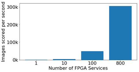
The resulting services can then be called by any gRPC client. To score our full dataset as quickly as possible, we created 800 identical instances of this FPGA service, each with its own dedicated FPGA.
Scoring Client Application and Infrastructure
We provisioned dedicated scoring VMs to load input images and formulate FPGA service requests as quickly as possible. We chose to use DS64_v3 Azure VMs because they offer a combination of fast I/O from managed disks and 64 cores for compute-intensive workloads. We created a multithreaded C# scoring client application to handle multiple requests to the same FPGA service in parallel and found that twenty scoring client threads were needed to maximize response throughput from a single FPGA service. This illustrates that the FPGA service can handle many concurrent requests by performing many tasks (like image preprocessing and Keras layer application) in parallel on the CPU, ensuring optimal use of the FPGA.
By running multiple instances of this client, we found that we were able to saturate multiple FPGA services using a single scoring VM; however, response rate eventually became IO-bound when many instances of the client were attempting to read from managed disk concurrently. We explored reading images from mounted blob containers rather than managed disks: this improved our I/O rate scaling during concurrent access, but unfortunately introduced additional latency. We therefore modified the scoring client to load 10k batches from disk and then score them after loading was complete, allowing us to separately time loading vs. scoring. With this arrangement, we can saturate ten FPGA services per scoring VM before response rate per service began to drop due to full CPU utilization on scoring VMs.
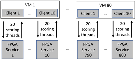
To fully saturate all 800 FPGA services, we created 80 VMs, each using 10 instances of the scoring client to score against 10 different FPGA services. These VMs and copies of the appropriate data disks were created using a PowerShell script and setup/orchestration scripts run remotely via PuTTY.
Results
We used the total time spent scoring by the slowest scoring client instance – 10 minutes, 38 seconds – as the "duration" of the scoring run. (The wall time of the scoring run, including image loading from disk, was ~47 minutes.) About 195 million images were scored during this time, at a rate of ~305k images per second.
Our results were highlighted in Ignite sessions by Joseph Sirosh, Doug Burger and Ted Way, Mark Russinovich and Haishi Bai, and Jennifer Marsman, using a graphical visualization and demo Python notebook for model training, FPGA service creation, and scoring.
Please see Lucas Joppa's recent blog post for more information on AI for Earth's FPGA Land Cover Mapping project. For more information on Project Brainwave, please see the GitHub repository and recent preview announcement.
Mary, Daniel, Xiaoyong, Wilson, Erika & Wee Hyong