Embarrassingly Parallel Image Classification, Using Cognitive Toolkit and TensorFlow on Azure HDInsight Spark
This post is by Mary Wahl, Data Scientist, T.J. Hazen, Principal Data Scientist Manager, Miruna Oprescu, Software Engineer, and Sudarshan Raghunathan, Principal Software Engineering Manager, at Microsoft.
Summary
Deep neural networks (DNNs) are extraordinarily versatile and increasingly popular machine learning models that require significantly more time and computational resources for execution than traditional approaches. By deploying these models on Microsoft HDInsight clusters, data scientists and engineers can easily scale available computation resources to achieve a desired throughput rate while using familiar scripting languages and deep learning frameworks. In this blog post, the fifth in our series showcasing deep learning applications on Azure, we show how DNNs produced in two common deep learning frameworks, Microsoft's Cognitive Toolkit (CNTK) and Google's TensorFlow, can be operationalized for scoring large image collections harbored on Azure Data Lake Store using PySpark. We apply this approach to a common DNN use case – aerial image classification – and demonstrate how the method can be used to identify recent patterns in urban development.
This blog post is a short summary of our work. Please see the full tutorial for sample data/code/models and step-by-step walkthroughs.
The previous four blog posts in this series, listed below, cover training and operationalization of DNNs with other deep learning frameworks, scripting languages, use cases, and/or Azure services. All four posts utilize MXNet, an alternative deep learning framework to CNTK and TensorFlow. Whereas the work highlighted in this post uses Python/PySpark, posts 1-3 showcase Microsoft R Server/SparkR. Post 4 discusses the training of a text classification model and its operationalization on Azure Web Apps (rather than HDInsight Spark).
- Building Deep Neural Networks in the Cloud with Azure GPU VMs, MXNet and Microsoft R Server
- Applying Deep Learning at Cloud Scale, with Microsoft R Server & Azure Data Lake
- Training Deep Neural Networks on ImageNet Using Microsoft R Server and Azure GPU VMs
- Cloud-Scale Text Classification with Convolutional Neural Networks on Microsoft Azure
Description of the Aerial Image Classification Use Case
The classification of aerial images is a common task with significant economic and political impact across a wide range of industries. Aerial photography is often analyzed in precision agriculture to monitor crop performance and identify regions in need of corrective treatments. In marketing and finance, image classifiers can identify property features and aid in property value estimation. Government agencies may use aerial imagery classification to enforce regulations: for example, Greece recently uncovered tens of thousands of tax evaders by identifying properties containing home pools. Image classifiers are also employed in geopolitical surveillance to identify novel remote settlements, and to estimate population density or infer economic vitality when direct data are unavailable. Researchers in government in academia may also use aerial data to track urban expansion, deforestation, and the impact of climate change.
This blog post and the associated tutorial focus on a specific use case: predicting a region's land use type (developed, cultivated, forested etc.) from aerial imagery. Large training and validation datasets for this application can easily be constructed from the vast troves of regularly-published and freely-available U.S. aerial images and ground-truth land use labels. Image classifiers trained on this data can quantify trends in land use and even identify new land development at the level of individual properties, as we will illustrate below.
Training Aerial Image Classifiers Through Transfer Learning
Producing a DNN from scratch can require weeks of GPU compute time and extraordinarily large training datasets. A common alternative is to repurpose an existing DNN trained to perform a related task: this process is called transfer learning or retraining. To illustrate how transfer learning is performed, we introduce the DNN architecture of AlexNet (a prototypical image classification DNN employed in this use case) and the practical role of each layer.
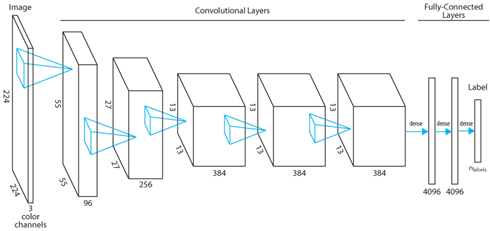
The first layer in AlexNet (and most other image classification DNNs) is a convolutional layer. Each neuron in the layer takes as input data from an 11 pixel x 11 pixel x 3 color channel (RGB) region of the input image. The neuron's learned weights, which are collectively referred to as its convolution filter, determine the neuron's single-valued output response to the input. A convolution with dimensions 55 x 55 x 1 could be produced between the neuron's filter and the full 224 x 224 x 3 input image by sliding the input region along the image's x and y dimensions in four-pixel strides. In practice, the equivalent convolution is normally implemented by statically connecting 55 x 55 identical copies of the neuron to different input regions. Ninety-six such sets of neurons make up the first layer of AlexNet, allowing 96 distinct convolution filters to be learned.
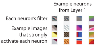
During training, many of the neurons in the first layer learn convolution filters that correspond to edge detectors, each potentially with a different orientation and/or color sensitivity. This functionality can be visualized either by examining the convolution filters themselves or by identifying images that would strongly activate the neuron, a technique pioneered by Zeiler & Fergus (2013). The image below, reproduced with permission from Matt Zeiler, shows the convolution filter (top) and sample strongly-activating images (bottom) for four example neurons in the first layer of AlexNet:
Typical image classification DNNs contain additional convolutional layers that combine the output of first-layer neurons to identify more complex shapes. Sample images that strongly activate example neurons in the second through fifth layer of a trained DNN are shown below (reproduced with permission from Matt Zeiler). Neurons in lower layers are strongly activated by simple shape and color combinations that may be present in images of many labels, such as round objects or legs. In higher layers, neurons are often more class-specific: they may be activated by the same object viewed from multiple perspectives, or by different objects with the same label.
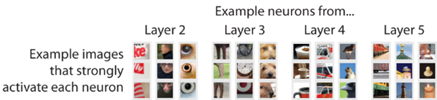
The complex shapes identified by later convolutional layers are excellent predictors of an image's classification, but are most effective in combination. For example, "tire" shapes may be present in images of cars and motorcycles, but an image that contains both "tire" and "helmet" shapes probably depicts a motorcycle. The fully-connected layers that typically follow convolutional layers in image classification DNNs encode such logic in the trained model. The model's final fully-connected layer comprises a number of neurons equal to the number of classes (1000, for the original AlexNet); the model's predicted output label is given by the index of the maximally-activated neuron in this layer.
In transfer learning, a pretrained model's final layer (and, sometimes, more of the fully-connected layers) is removed and replaced with a new layer/layers that will be trained for the new classification task. In the simplest form of transfer learning, the trained model's preserved layers are "frozen": no changes are made to their weights during retraining. This reduces the potential for overfitting by limiting the number of free parameters in the model, but creates image features that may not be ideally suited for the new image classification task. An alternative method called fine-tuning allows updates to the old layers' weights, which better adapts featurization for the new task but typically requires a larger training set to avoid overfitting.
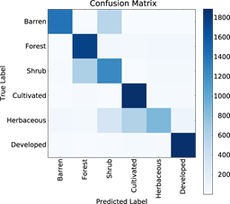
To train our aerial image classifiers, we replaced the final layers from ImageNet-trained image classification DNNs (AlexNet for CNTK, a 50-layer ResNet for TensorFlow) and froze the remaining layers. We were delighted to find that the features developed to distinguish the categories in ImageNet were suitable even for the apparently unrelated task of classifying aerial imagery. (Overall accuracy for both models was ~80% across six land use categories, rising to ~92% when undeveloped land categories were grouped together; the confusion matrix for the CNTK model is shown below.) Many others have also reported improbable efficacy for models developed through transfer learning: such anecdotal successes, combined with relatively low resource requirements and the ability to tolerate small training sets, explains why transfer learning is now far more common in industrial applications than de novo model training.
Operationalization on Spark
Data scientists commonly employ a method called minibatching during DNN training. In this approach, a subset of the available training images are scored in each training round (usually in parallel across many cores of a GPU), and the results are combined to better infer a gradient for parameter updates. Most deep learning frameworks, including CNTK and TensorFlow, implement minibatching with handy methods to describe how training files should be loaded and preprocessed. Users would be remiss not to take advantage of these efficient functions during training, but may be unable to use them when applying the trained model to new data. Our use case, for example, requires applying the trained DNNs to large image sets on Azure Data Lake Store using PySpark: in this context, the built-in image loading/preprocessing in CNTK and TensorFlow can't be used because the files are not stored locally. (The same issue arises e.g. in many web service and robotics applications.) It is necessary in such circumstances to faithfully replicate the loading and preprocessing steps that were performed during model training. Example Python scripts illustrating the details of this process are available in the associated Git repository.
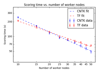
Deep learning framework installation and adaptations to evaluation scripts for parallelization are also important considerations for operationalizing DNNs on Spark clusters. We provide an example script action to coordinate the installation of CNTK, TensorFlow, and all dependencies. Spark clusters are designed to quickly perform distributable tasks by assigning a proportion of the workload to each "worker node": the number of worker nodes can be specified during deployment and dynamically scaled later to accommodate changing needs. As shown below, the total time required to execute the image processing task scales inversely with the number of nodes available for processing. The colocation of the Spark cluster on the same Azure Data Lake Store as the input data and a rational choice of image partitioning across workers reduced the load latency for both images and models. Sample Jupyter notebooks included in our tutorial illustrate the specifics of our image processing coordination using PySpark.
Applications of the Aerial Image Classifier
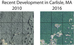
To demonstrate the potential uses of our trained classifier, we applied the CNTK model to aerial images tiling Middlesex County, MA (home of Microsoft's New England Research and Development Center). Comparing the model's predictions on images collected in 2016 to the most recent available ground-truth labels (from 2011) allowed us to identify newly-developed areas in the county, including single properties in some cases (see center 224 meter x 224 meter tile below).
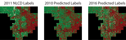
The accuracy of our model was also sufficient to capture the major trends in urban development across the county. In the figure below, each pixel represents the classification of a single 224 meter x 224 meter region, with green pixels representing undeveloped land, red pixels representing developed land, and white pixels representing cultivated land. (The ground-truth labels from the National Land Cover Database are provided at left; predictions on contemporary and more recent aerial images are shown at center and right, respectively.)
For a more detailed description of our work, including sample data/code and walkthroughs, please check out the associated tutorial.
Mary, T.J., Miruna & Sudarshan
Our thanks to Mario Bourgoin, Yan Zhang and Rahee Ghosh for proofreading and test-driving the tutorial accompanying this blog post.