Cognitive Toolkit Helps Win 2016 CIF International Time Series Competition
This post is authored by Slawek Smyl, Senior Data & Applied Scientist at Microsoft.
The Computational Intelligence in Forecasting (CIF) International Time Series Competitionwas one of ten competitions held at the IEEE World Congress on Computational Intelligence (IEEE WCCI) in Vancouver, Canada, in late July this year. I am excited to report that my CIF submission won the first prize! In this blog post, I would like to provide an overview of:
- The CIF competition.
- My winning submission and its algorithms.
- The tools I used.
CIF International Time Series Competition
This competition started in 2015 with the goal of getting an objective comparison of existing and new Computational Intelligence (CI) forecasting methods (Stepnicka & Burda, 2015). The IEEE Computational Intelligence Society defines these methods as "biologically and linguistically motivated computational paradigms emphasizing neural networks, connectionist systems, genetic algorithms, evolutionary programming, fuzzy systems, and hybrid intelligent systems in which these paradigms are contained" (IEEE Computational Intelligence Society, 2016).
In the CIF 2016 competition, there were 72 monthly time series of medium length (up to 108-long). 24 of them were bank risk analysis indicators, and 48 were generated. In a large majority of cases, the contestants were asked to forecast 12 future monthly values (i.e. up to 1 year ahead), but for some shorter series, the forecasting horizon was smaller, at 6 future values.
The error metric was the average sMAPE over all time-series. The sMAPE for a single time series is defined as below:
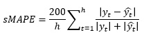
where h is the maximum forecasting horizon (6 or 12 here),  is a true value at the horizon t, and
  is the forecast for the horizon t.
Up to 3 submissions, without feedback, were allowed.
Four statistical methods were used for the purposes of comparison – Exponential Smoothing (ETS), ARIMA, Theta and Random Walk (RW), and two ensembles using simple and Fuzzy Rule based averages.
Winning Submission, Algorithms & Results
The organizers received 19 submissions from 16 participants: 8 NN-based, 3 fuzzy, 3 hybrid methods, and 2 others (kernel-based, Random Forest). Interestingly, Computational Intelligence methods performed relatively better on real as opposed to generated time series: on the real life series, the best statistical method was ranked 6th. On the generated time series, a statistical algorithm called "Bagged ETS" won. One can speculate that this is because statistical algorithms generally assume a Gaussian noise around a true value, but this assumption is incorrect for many "real-life" series, e.g. they tend to have "fatter" tails, in other words, the probability of outliers is higher. Overall, two of my submissions got 1st and 2nd places. I will describe now my winning submission, a Long Short-Term Memory (LSTM) based neural network applied to de-seasonalized data.
Data Preprocessing
Forecasting time series with Machine Learning algorithms or Neural Networks is usually more successful with data preprocessing. This is typically done with a moving (or "rolling") window along the time series. At each step, constant size features (inputs) and outputs are extracted, and therefore each series can be a source of many input/output records. For networks with squashing functions like sigmoid, a normalization is often helpful, and it is more needed if one tries to train a single network of this kind on many time series differing in size (amplitude). Finally, for seasonal time series, although in theory a neural network should be able to deal with them well, it often pays off to remove the seasonality during the data preprocessing step.
All the above was present in the preprocessing used by my winning submission. It started with applying logarithm and then the stl() functions of R. STL decomposes a time series into seasonal, trend, and irregular components. The logarithm transformation provides two benefits: firstly, it is part of the normalization, secondly, it converts the STL's normally additive split into a multiplicative one (remember that log (x+y) = log (x) * log (y)), and the multiplicative seasonality is a safer assumption for non-stationary time series. The graph in Figure 1 illustrates this decomposition.
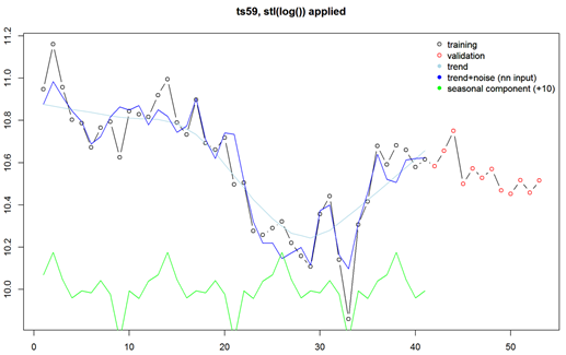
Figure 1
So, after subtracting the seasonality, the moving window was applied to cover 15 months (points) in case of the 12 months' ahead forecast. It's worth stressing that the input is a 15-long vector and the output is a 12-long vector, so we are forecasting the whole year ahead at once. This approach works better than trying to forecast just one month ahead – to get the required 12-step (month) ahead forecast, one would need to forecast 12 times, and use the previous forecast as input 11 times. That leads to instability of the forecast.
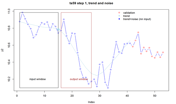
Figure 2
Then, the last value of trend inside the input window (the big filled dot above) is subtracted from all input and output values for normalization. The values are stored as part of this time series sequence. Input and output windows move forward one step and the normalization step is repeated. Two files are created: training and validation. The procedure described above continues until the last point of the input window is positioned at lengthOfSeries-outputSize-1, e.g. here 53-12, in case of the training file, or until the last point of the output window equals the last point of the series, in case of the validation file. The validation file contains the training file, but actually only the last record of each series is used – the rest, although later forecasted, is discarded and only used as a "warm-up" region for the recurrent neural network used (LSTM).
The data preprocessing described here is relatively simple, it could have been more sophisticated, e.g. one could use some artifacts of other statistical algorithms like Exponential Smoothing as features.
Neural Network Architecture
A typical time series preprocessing as described above has an obvious weakness: data outside of the input window has no influence on the current derived features. Such missing information may be important. On the other hand, extending the size of the input window may not be possible due to the shortness of the series. This problem can be mitigated by using Recurrent Neural Networks (RNN) – these have internal directed cycles and can "remember" some past information. LSTM networks (Hochreiter & Schmidhuber, 1997) can have a long memory and have been successfully used in speech recognition and language processing over the last few years. The winning submission used a single LSTM network (layer) and a simple linear "adapter" layer without bias. The whole solution is shown in Figure 3 below.
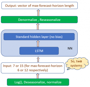 Figure 3
Microsoft Cognitive Toolkit and R
The neural network was run using Microsoft Cognitive Toolkit, formerly known as CNTK (Microsoft, 2016). Cognitive Toolkit is Microsoft's Open Source neural network toolkit, available for Windows and Linux. It is highly scalable and can run on a CPU, one or more GPUs in a single computer, and on a cluster of servers, each running several GPUs. This scalability was actually not needed for this project – the entire learning took just a few minutes on a PC with a single GPU. However, the ease of creation and experimentation with neural networks architectures was the highlight. Microsoft Cognitive Toolkit shines here – it allows you to express almost arbitrary architectures, including recurrent ones, through mathematical formulas describing the feed-forward flow of the signal. For example, the figure below shows the beginning of the definition of an LSTM network; note how easy it is to get a past value for a recurrent network, and how straightforward the translation from mathematical formulas to code. Preprocessing and post-processing was done with R.
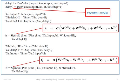
Figure 4
Please note that, in my current implementation of the system described in the Cortana Intelligence Gallery tutorial, you will not find the formulas shown in Figure 4. I rewrote my original script that utilizes a preconfigured LSTM network (September 2016, Microsoft Cognitive toolkit version 1.7). The configuration file is much simpler now and you can access it here. To download the dataset, visit https://irafm.osu.cz/cif.
Slawek
Bibliography
Hochreiter, S. & Schmidhuber, J., 1997. Long short-term memory. Neural Computation, 9(8), p. 1735–1780.
IEEE Computational Intelligence Society, 2016. Field of Interest. [Online]
Available at: https://cis.ieee.org/field-of-interest.html
Microsoft, 2016. CNTK. [Online]
Available at: https://github.com/Microsoft/CNTK
Stepnicka, M. & Burda, M., 2015. Computational Intelligence in Forecasting – The Results of the Time Series Forecasting Competition. Proc. FUZZ-IEEE.
Stepnicka, M. & Burda, M., n.d. [Online]
Available at: https://irafm.osu.cz/cif