Training Deep Neural Networks on ImageNet Using Microsoft R Server and Azure GPU VMs
This post is by Miguel Fierro, Data Scientist, Max Kaznady, Data Scientist, Richin Jain, Solution Architect, Tao Wu, Principal Data Scientist Manager, and Andreas Argyriou, Data Scientist, at Microsoft.
Deep learning has made a lot of strides in the computer vision subdomain of image classification in the past few years. This success has opened up many use cases and opportunities in which Deep Neural Networks (DNNs) similar to the ones used in computer vision can generate lots of business value, and in a wide range of applications including security (e.g. identifying luggage at airports), traffic management (identifying cars), brand tracking (tracking how many times the brand logo on a sportsperson's apparel appears on TV), intelligent vehicles (classifying traffic signals or pedestrians), and many more.
These advances are becoming possible because of a couple of reasons: DNNs are able to classify objects in images with high accuracy (more than 90%, as we will show in this post) and also because we have access to cloud resources such as Azure infrastructure which allow us to operationalize image classification in a highly secure, scalable and efficient way.
This is the third post in our cloud deep learning blog series featuring Microsoft R Server, MXNet and Azure cloud computing components. In our first post, we showed how to set up cloud deep learning using Azure N-series GPU VMs and Microsoft R Server. In the second post, we demonstrated an end-to-end cloud deep learning workflow and parallel DNN scoring using HDInsight Spark and Azure Data Lake Store.
In this latest post, we demonstrate how to utilize the computing power offered by multiple GPUs in Azure N-Series VMs to train state-of-the-art deep learning models on complex machine learning tasks. We show training and scoring using deep residual learning, which has surpassed human performance when it comes to recognizing images in databases such as ImageNet.
ImageNet Computer Vision Challenge
The ImageNet Large Scale Visual Recognition Competition (ILSVRC), which began in 2010, has become one of the most important benchmarks for computer vision research in recent years. The competition has three categories:
- Image classification: Identification of object categories present in an image.
- Single object localization: Identifying a list of objects present in an image and drawing a bounding box showing the location of one instance of each object in the image.
- Object detection: Similar to single object location above, but with the added complexity of having to draw bounding boxes around every instance of each object.
In this post, we focus on the first task of image classification.
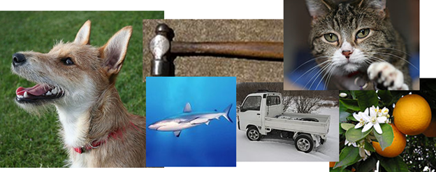
Figure 1: Some of the classes annotated in the ImageNet dataset (images from Wikipedia).
The ImageNet image dataset used in ILSVRC competition contains objects annotated according to the WordNet hierarchy (Figure 1). Each object in WordNet is described by a word or group of words called "synonym set" or "synset". For example: "n02123045 tabby, tabby cat", where "n02123045" is the class name and "tabby, tabby cat" is the description. ILSVRC uses a subset of this dataset, and specifically we are using an ILSVRC subset from 2012, which contains 1000 classes of images.
The ImageNet data for the competition is further split into the following three datasets:
- Training set with 1000 classes and roughly 1200 images for each class (up to 1300 images per class), which is used to train the network (1.2 million images in total).
- Validation set of 50,000 images, sampled randomly from each class. It is used as the ground truth to evaluate the accuracy of each training epoch.
- Test set of 100,000 images selected randomly from each class. It is used to evaluate the accuracy in the competition and to rank the participants.
Training the Microsoft Research Residual DNN with Microsoft R Server and Four GPUs
The Residual Network (ResNet) architecture, introduced in 2015 by Microsoft Research (MSR), has made history as the first DNN to surpass human performance in the complex task of image classification. DNNs in the computer vision domain have been extremely successful, because they can learn hierarchical representations of an image: each layer learns successively more complex features. When stacked together, the layers are capable of very complex image identification tasks. Examples of simpler features include edges and regions of an image, whereas a good example of a more advanced feature which a DNN can learn would be one part of an object, e.g. the wheel of a car.
A DNN with a higher number of layers can learn more complex relationships but also becomes more difficult to train using optimization routines such as Stochastic Gradient Descent (SGD). The ResNet architecture introduces the concept of residual units which allow very deep DNNs to be trained: SGD attains successively better performance over time and eventually reaches convergence.
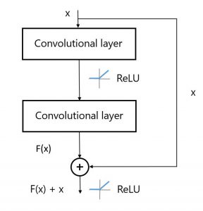 Figure 2: Schema of a residual unit.
The idea of residual units is presented in Figure 2. A residual unit has one or more convolution layers, labeled as F(x), and adds to these the original image (or output of the previous hidden layer), F(x) + x. The output of a residual unit is therefore a hierarchical representation of the image, produced by the convolutions and the image itself. ResNet authors believe that "it is easier to optimize the residual mapping than to optimize the original, unreferenced mapping". The authors presented a DNN of 152 layers in 2015 – the deepest architecture to-date.
Training an 18-layer ResNet with 4 GPUs
We showcase the training of ResNet in one of our Azure N-series GPU VMs (NC24), which has four NVIDIA Tesla K80 GPUs. We implemented our own 18-layer ResNet network (ResNet-18 for short) using the MXNet library in Microsoft R Server – the full implementation is available here. We chose the smallest 18-layer architecture for demo purposes as it minimizes the training time (a full 152-layer architecture would take roughly 3 weeks to train). ResNet-18 is also the smallest architecture which can be trained to result in decent accuracy. There are other layer combinations which can be created: 34, 50, 101, 152, 200 and 269. The implemented architecture is based on ResNet version 2, where the authors reported a 200-layer network for ImageNet and a 1001-layer network for the CIFAR dataset.
The MXNet library natively supports workload partitioning and parallel computation across the 4 GPUs of our Azure N-series GPU VM. The images are supplied to the training process via an iterator, which allows the loading of a batch of images in memory. The number of images in the batch is called batch size. The neural network weight update is performed in parallel across all four GPUs. The memory consumed by the process on each GPU (Figure 3) depends on the batch size and the complexity of the network.
The learning rate has a large effect on the algorithm performance – too fast and the algorithm won't converge, but too slow and the algorithm will take a significant amount of training time. For large problems such as the one we are discussing, it is important to have a schedule for reducing the learning rate according to the epoch count. There are two methods which are commonly used:
- Multiply the learning rate by a factor smaller than one at the end of every epoch.
- Keep the learning rate constant and decrease by a factor at certain epochs.
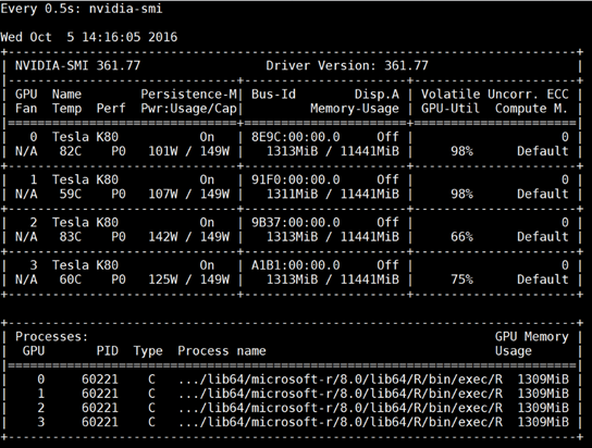
Figure 3: GPU memory consumption and utilization while training ResNet-18 on 4 GPUs with a batch size of 144.
During training, we used the top-5 accuracy (instead of using the top-1 accuracy), which does not record misclassification if the true class is among the top 5 predictions. The prediction output for each image is a vector of size 1000 with the probability of each of the 1000 classes. The top-5 results are the 5 classes with the highest probability. The use of top-5 accuracy was initially set in the ImageNet competition due to the difficulty of the task and it is the official ranking method.
It takes roughly 3 days to train ResNet-18 for 30 epochs in Microsoft R Server on an Azure N-series NC-24 VM with four GPUs. The top-5 accuracy at epoch 30 is 95.02% on the training set and 91.97% on the validation set. Training progress is displayed in Figure 4.
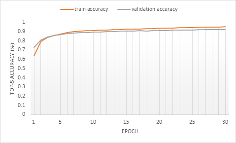
Figure 4: Top-5 accuracy on the training set and validation set.
To better visualize the results, we created a top-5 accuracy confusion matrix (Figure 5). The matrix size is 1000 by 1000, corresponding to the 1000 classes of ImageNet. The rows correspond to the true class and the columns to the predicted class. The matrix is constructed as a histogram of the predictions. For each image, we represent the pair (true label, prediction k) for the k=1,…,5 predictions. The bright green represents a high value in the histogram and the dark green represents a low value. Since the validation set consists of 50,000 images, we produce a matrix of 250,000 elements. We used the visualization library datashader and the trained ResNet-18 model at epoch 30.
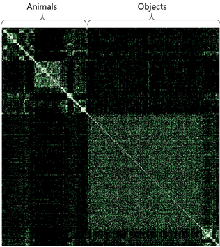 Figure 5: Confusion matrix of top-5 accuracy in ResNet-18 using the validation set at epoch 30. The rows represent the real class and the columns the predicted class. A bright green represents a high density of points, while a dark green represents a low density.
The diagonal line in the confusion matrix represents perfect predictor with zero misclassification rate – the predicted class exactly matches the ground truth. Its brightness shows that most images are correctly classified among the top-5 results (in fact more than 90% of them).
In Figure 5, we observe that there are two distinct clusters of points: one corresponding to animals another to objects. The animal group contains several clusters, while the group corresponding to objects is more scattered. This is because in the case of animals, certain clusters represent groups from the same species (fish, lizards, birds, cats, dogs, etc.). In other words, if the true class is a golden retriever, it is better for our model to classify the image as another breed of dog than as a cat. For objects, the misclassifications are more sporadic.
We can visualize how the results change as the number of epochs increases. This is represented in the Figure 6, where we create a matrix with the model from epoch 1 to 30 and the images in the validation set.
Figure 6: GIF of the evolution of the top-5 accuracy in ResNet-18 using the validation set and epochs 1 to 30.
Operationalizing Image Classification with MXNet and Microsoft R Server
We can now use the model we have just trained to identify animals and objects in images that belong to one of the 1000 classes in our dataset, which can be done with high accuracy as indicated by our results.
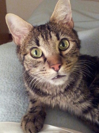
Figure 7: Neko looking surprised.
As an example we can try to predict the class of our little friend Neko in Figure 7. We obtain a good-enough prediction at epoch 28:
Predicted Top-class: "n02123045 tabby, tabby cat"
Top 5 predictions:
[1] "n02123045 tabby, tabby cat"
[2] "n02124075 Egyptian cat"
[3] "n02123159 tiger cat"
[4] "n02127052 lynx, catamount"
[5] "n02125311 cougar, puma, catamount, mountain lion, painter, panther, Felis concolor"
As we can see, the prediction is very accurate, classifying Neko as a tabby cat. Not only that, but also the rest of the Top-5 results are cat-like animals. This result and the analysis of the clusters in the confusion matrix of Figure 5 suggest that the network is in some degree learning the global concept of each class in the images. Clearly, it is better for the network to misclassify Neko as an Egyptian cat than as an object.
All the code for ResNet training and prediction on ImageNet can be accessed via this repo.
Summary
We showed how to train ResNet-18 on the ImageNet dataset using Microsoft R Server and Azure N-series GPU VMs. You can experiment with different hyper-parameter values and even train ResNet-152 to surpass human accuracy using our Open Source implementation.
We would like to highlight once again that it's not only important to achieve high Top-1 accuracy, but also that Top-5 misclassifications have to be related to the true class. Our results show that the network is learning to differentiate animals from objects, and even learn the concept of species within animals.
We can easily operationalize the trained model with a framework similar to the one we described in our previous blog post. In our next post, we will focus on adjacent domains where deep learning can be applied, such as in textual data.
Miguel, Max, Richin, Tao & Andreas.