Building Azure ML Models on the NYC Taxi Dataset

This blog post is by Girish Nathan, a Senior Data Scientist at Microsoft.

The NYC taxi public dataset consists of over 173 million NYC taxi rides in the year 2013. The dataset includes driver details, pickup and drop-off locations, time of day, trip locations (longitude-latitude), cab fare and tip amounts. An analysis of the data shows that almost 50% of the trips did not result in a tip, that the median tip on Friday and Saturday nights was typically the highest, and that the largest tips came from taxis going from Manhattan to Queens.

This post talks about Azure ML models that we built on this data, with the goal of understanding it better.

Problem Statement

We categorized tip amounts into the following five bins:

Although there are several ML problems that this dataset can be used for, we focused on the following problem statement:

Given a trip and fare - and possibly other derived features - predict which bin the tip amount will fall into.

We can model this as a multiclass classification problem with 5 classes. An alternative is ordinal regression, which we do not discuss here. An Azure ML technology we used is Learning with Counts (aka Dracula) for building count features on the categorical data, and a multiclass logistic regression learner for the multiclass classification problem.

The Dataset

The NYC taxi dataset is split into Trip data and Fare data. Trip data has information on driver details (e.g. medallion, hack license and vendor ID), passenger count, pickup date and time, drop off date and time, trip time in seconds and trip distance. Fare data has information on the trip fare, relevant tolls and taxes, and tip amount.

An excerpt of the datasets is shown below.

Trip data example:

Schema:  
medallion,hack_license,vendor_id,rate_code,store_and_fwd_flag,pickup_datetime,
dropoff_datetime,passenger_count,trip_time_in_secs,trip_distance,
pickup_longitude,pickup_latitude,dropoff_longitude,dropoff_latitude

Example:
89D227B655E5C82AECF13C3F540D4CF4,BA96DE419E711691B9445D6A6307C170,CMT,1,N,2013-01-01 15:11:48,2013-01-01 15:18:10,4,382,1.00,-73.978165,40.757977,-73.989838,40.751171

Fare data example:

Schema:
medallion,hack_license,vendor_id,pickup_datetime,payment_type,fare_amount,
surcharge,mta_tax,tip_amount,tolls_amount,total_amount

Example:
89D227B655E5C82AECF13C3F540D4CF4,BA96DE419E711691B9445D6A6307C170,CMT,2013-01-01 15:11:48,CSH,6.5,0,0.5,0,0,7

Data Preprocessing

We perform a join operation of the Trip and Fare data on the medallion, hack_license, vendor_id, and pickup_datetime to get a dataset for building models in Azure ML. We then use this dataset to derive new features for tackling the problem.

Derived Features

We preprocess the pickup date time field to extract the day and hour. This is done in an Azure HDInsight (Hadoop) cluster running Hive. The final variable is of the form “day_hour” where day takes values from 1 = Monday to 7 = Sunday and the hour takes values from 00 to 23. We also use the hour to extract a categorical variable called “that_time_of_day” – this takes 5 values, Morning (05-09), Mid-morning(10-11), Afternoon(12-15), Evening(16-21), and Night(22-04).

Since the data has longitude-latitude information on both pickup and drop-off, we can use this in conjunction with some reverse geocoding software (such as this one, provided by the Bing Maps API) to derive a start and end neighborhood location and code these as categorical variables. These new features are created to reduce the dimensionality of the pickup-drop-off feature space and they help in better model interpretation.

Dealing with High Dimensional Categorical Features

In this dataset, we have many high dimensional categorical features. For example, medallion, hack_license, day_hour and also raw longitude-latitude values. Traditionally, these features are dealt with by one-hot encoding them (for an explanation, click here). While this approach works well when the categorical features have only a few values, it results in a feature space explosion for high dimensional categorical features and is generally unsuitable in such contexts.

An efficient way of dealing with this is using Learning with Counts to derive conditional counts based on the categorical features. These conditional counts can then be directly used as feature vectors or transformed into something more convenient.

Deriving Class Labels for the Multiclass Classification Problem

We map the tip amounts into the 5 bins mentioned in the Problem Statement above using an Execute R module in Azure ML and then save the train and test data for further use.

Model Building in Azure ML

After subsampling the data so that Azure ML can consume it, we are ready to build models for the problem at hand.

Class Distributions in Train Dataset

For our training data, the class distributions are as follows:

Class 0 : 2.55M examples (49%)
Class 1 : 2.36M examples (45%)
Class 2 : 212K examples (4.1%)
Class 3 : 65K examples (1.2%)
Class 4 : 26K examples (0.7%)

Modeling the Problem Using Learning with Counts, and Experimental Results

As mentioned in the earlier blog post on Learning with Counts, using conditional counts requires building count tables on the data. In our case, we split our final dataset into three components: One for building count tables, another for the training of the model, and a third for the test dataset. Once count features are built using the data allocated for building count tables, we featurize our train and test datasets using those count features.

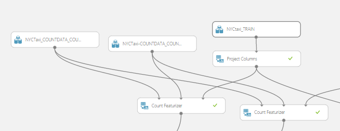
We show a sample of the experiment to illustrate the set-up:

The Build Count Table module builds a count table for the high dimensional categorical features on a 33GB dataset allocated for counts using MapReduce. We then use those count features in the Count Featurizer module to featurize the train, test, and validation datasets. As is standard practice, we use the train and validation datasets for parameter sweeps, and then use the “best learned model” to score on the test dataset. This part of the experiment is shown below:

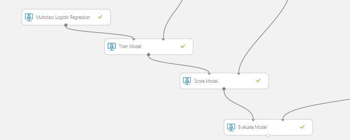
The model training and scoring portion of the experiment looks like so: 

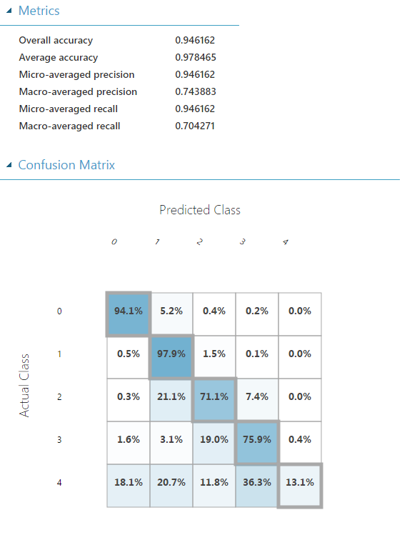
We can now use a standard confusion matrix to summarize our results. As is common, the rows represent the true labels and the columns the predicted labels.

Modeling the Problem Without Learning with Counts, and Experimental Results

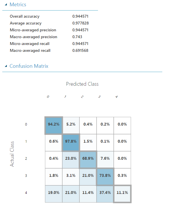
For comparison, we show the results of using a multiclass logistic regression learner on data where feature hashing is used for reducing the dimensionality of the categorical features. The resulting confusion matrix on the test dataset is as follows:

Conclusion

We see that the use of conditional counts results in a higher prediction accuracy for the more rare classes. This accuracy benefit is likely due to the use of count tables to produce compact representations of high dimensional categorical features and was helpful in building better models for the NYC taxi dataset. When count features are not used, the high dimensional representation of the categorical features results in a higher variance model for the more rare classes as they have less data available for learning.

An additional benefit of using count features is that both the train and test times are reduced. For instance, for the NYC taxi dataset, we find that the model building time using count features is half of that without using count features. Similarly, the scoring time is also about half due to more effective featurization. This can be another significant benefit when dealing with large datasets.

Girish