Convolutional Neural Nets in Net#
This blog post is authored by Alexey Kamenev, Software Engineer at Microsoft.
After introducing Net# in the previous post, we continue with our overview of the language and examples of convolutional neural nets or convnets.
Convnets have become very popular in recent years as they consistently produce great results on hard problems in computer vision, automatic speech recognition and various natural language processing tasks. In most such problems, the features have some geometric relationship, like pixels in an image or samples in audio stream. An excellent introduction to convnets can be found here:
https://www.coursera.org/course/neuralnets (Lecture 5)
https://deeplearning.net/tutorial/lenet.html
Before we start discussing convnets, let’s introduce one definition that is important to understand when working with Net#. In a neural net structure, each trainable layer (a hidden or an output layer) has one or more connection bundles. A connection bundle consists of a source layer and a specification of the connections from that source layer. All the connections in a given bundle share the same source layer and the same destination layer. In Net#, a connection bundle is considered as belonging to the bundle's destination layer. Net# supports various kinds of bundles like fully connected, convolutional, pooling and so on. A layer might have multiple bundles which connect it to different source layers.
For example:
// Two input layers. input Picture [28, 28]; input Metadata [100];hidden H1 [200] from Picture all; // H2 connected both to H1 and Metadata layers using different connection types hidden H2 [200] { from H1 all; // This is a fully-connected bundle. from Metadata where (s, d) => s < 50; // This is a filtered (sparse) bundle. } output Result [10] softmax from H2 all; |
Layer H2 has 2 bundles, one is fully connected and the other filtered. In such a scenario, defining layer H2 as just “fully connected” or “filtered” does not fully reflect the actual configuration of the layer, so that’s why we chose term “bundle” to describe connection types.
Now let’s talk about convnets. As in previous post, we will use the MNIST dataset. Let us start with a very simple convnet from the “Neural Network: Basic Convolution” sample. Sign up for our free trial to run this sample.
const { T = true; F = false; } input Picture [28, 28]; hidden C1 [5, 12, 12] from Picture convolve { InputShape = [28, 28]; // required KernelShape = [ 5, 5]; // required Stride = [ 2, 2]; // optional, default is 1 in all dimensions MapCount = 5; // optional, default is 1 } // Only part of the net shown, see the sample for complete net structure |
Hidden layer C1 has a convolutional bundle of the following configuration:
InputShape defines the shape of the source layer for the purpose of applying convolution. The product of the dimensions of InputShape must be equal to the product of the dimensions of source layer output but the number of dimensions does not have to match. For example, Picture layer can be declared as:
input Picture[784];
Receptive field is 5 by 5 pixels (KernelShape).
Stride is 2 pixels in each dimension. In general, smaller strides will produce better results but take more time to train. Larger strides will allow the net to train faster but may produce worse results.
Number of output feature maps is 5. The same will be the number of sets of weights (kernels or also known as filters).
No automatic padding.
Weights will be shared in both dimensions. That means there will be:
MapCount * (KernelShape[0] * KernelShape[1] + 1) = 130 total weights in this bundle (the “+ 1” term is for the bias which is a separate weight for each kernel).
Note that the C1 layer can be represented as 3-dimensional layer as it has five 2D-feature maps, each feature map of size 12 by 12. When automatic padding is disabled, the number of outputs in a particular dimension can be calculated using the following simple formula:
O = (I - K) / S + 1, where O is output, I – input, K – kernel and S – stride sizes.
For the layer C1:
O = (28 - 5) / 2 + 1 = 12 (using integer arithmetic)
Layer C2 is the next hidden layer with convolutional bundle that is connected to C1. It has a similar declaration except one new attribute, Sharing:
hidden C2 [50, 4, 4] from C1 convolve { InputShape = [ 5, 12, 12]; KernelShape = [ 1, 5, 5]; Stride = [ 1, 2, 2]; Sharing = [ F, T, T]; // optional, default is true in all dimensions MapCount = 10; } |
Note that weight sharing is disabled in Z dimension, let’s take a closer look on what happens in such a case. Our kernel is essentially 2D (KernelShape Z dimension is 1), however, the input is 3D, with InputShape Z dimension being 5, in other words we have 5 input feature maps, each feature map being 12 by 12. Suppose we finished applying the kernel to the first input feature map and want to move to the second input feature map. If sharing in Z dimension were true, we would use the same kernel weights for the second input map as we used for the first. However, the sharing is false which means a different set of weights will be used to apply the kernel in the second input map. That means we have more weights and larger model capacity (this may or may not be a good thing as convnets are usually quite tricky to train).
To see the difference, here is the layer C2 weight count with disabled Z sharing:
(KernelShape[1] * KernelShape[2] + 1) * InputShape[0] * MapCount = (5*5+1)*5*10 = 1300
In case of enabled Z weight sharing, we get:
(KernelShape[1] * KernelShape[2] + 1) * MapCount = (5*5+1)*10 = 260
If you run the sample it should finish in about 5 minutes providing an accuracy of 98.41% (or 1.59% error) which is a further improvement over the fully-connected net from the previous Net# blog post (98.1% accuracy, 1.9% error).
Another important layer type in many convnets is a pooling layer. A few pooling kinds are used in convnets – the most popular are max and average pooling. In Net#, a pooling bundle uses the same syntax as a convolutional bundle thus allowing the same level of flexibility in defining pooling topology. Note that the pooling bundles are non-trainable, that is, they don’t have weights that are updated during the training process as pooling just applies a fixed mathematical operation. To demonstrate the usage of a pooling bundle, we’ll take a convnet from the “Neural Network: Convolution and Pooling Deep Net” sample. This net has several hidden layers with both convolutional and pooling bundles and uses parameterization to simplify the calculation of input and output dimensions.
hidden P1 [C1Maps, P1OutH, P1OutW] from C1 max pool { InputShape = [C1Maps, C1OutH, C1OutW]; KernelShape = [1, P1KernH, P1KernW]; Stride = [1, P1StrideH, P1StrideW]; } |
Using the same convolutional syntax to define pooling allows us to create various pooling configurations, for example, maxout layers (which are essentially 3D max pooling layer + linear activation function in convolutional layer) and many others.
If you run the sample it should finish in about 25 minutes providing an accuracy of 98.89% (or 1.1% error) which is a further improvement over the basic convnet described previously.
One more feature of a Net# convolutional bundle is padding which can be either automatic (the Net# compiler decides how to pad) or precise (the user provides exact padding sizes). In the case of automatic padding (Padding optional attribute, default is false), the input feature maps will be automatically padded with zeroes in the specified dimension(s):
hidden C1 [16, 24, 24] rlinear from Image convolve { InputShape = [3, 24, 24]; KernelShape = [3, 5, 5]; Stride = [1, 1, 1]; Padding = [false, true, true]; MapCount = 16; } hidden P1 [16, 12, 12] from C1 max pool { InputShape = [16, 24, 24]; KernelShape = [1, 3, 3]; Stride = [1, 2, 2]; Padding = [false, true, true]; } |
Also note a few other Net# features shown in this example:
C1 layer uses a rectified linear unit (ReLU) activation function - rlinear. See the Net# guide for the complete list of supported activation functions.
Pooling bundle in P1 layer uses overlapped pooling: kernel size is 3 in both X and Y dimensions while stride is 2 in both dimensions, so the applications of pooling kernel will overlap.
When padding is enabled, a slightly different formula is used to calculate output dimensions:
O = (I - 1) / S + 1
For the layer P1:
O = (24 - 1) / 2 + 1 = 12 (using integer arithmetic)
While training a complex neural network it is important to monitor the progress and adjust the training parameters or network topology in case the training does not converge or converges poorly. To see the progress of neural net training in Azure ML, run an experiment and, when the Train Model module starts running, click on the “View output log” link in the Properties pane. You should see something like this:
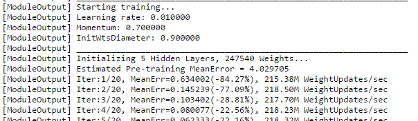
MeanErr is the mean training error and generally should be decreasing during the training process (it is ok for it to wiggle a bit from time to time). If it’s not decreasing, try changing training parameters (learning rate, initial weights diameter or momentum) or network architecture or both.
Try playing with these convnets and see what happens if you change:
Kernel size (for example to [3, 3] or [8, 8]).
Stride size.
Feature map count (MapCount).
Training parameters like learning rate, initial weights diameter, momentum and number of iterations.
A guide to Net# is also available in case you want to get an overview of most important features of Net#.
Do not hesitate to ask questions or share your thoughts – we value your opinion!
Alexey