Machine Learning, meet Computer Vision
This is part 1 of a 2 part series, co-authored by Jamie Shotton , Antonio Criminisi and Sebastian Nowozin of Microsoft Research, Cambridge, UK. The second part was later posted here.
Computer vision, the field of building computer algorithms to automatically understand the contents of images, grew out of AI and cognitive neuroscience around the 1960s. “Solving” vision was famously set as a summer project at MIT in 1966, but it quickly became apparent that it might take a little longer! The general image understanding task remains elusive 50 years later, but the field is thriving. Dramatic progress has been made, and vision algorithms have started to reach a broad audience, with particular commercial successes including interactive segmentation (available as the “Remove Background” feature in Microsoft Office), image search, face detection and alignment, and human motion capture for Kinect. Almost certainly the main reason for this recent surge of progress has been the rapid uptake of machine learning (ML) over the last 15 or 20 years.
This first post in a two-part series will explore some of the challenges of computer vision and touch on the powerful ML technique of decision forests for pixel-wise classification.
Image Classification
Imagine trying to answer the following image classification question: “Is there a car present in this image?” To a computer, an image is just a grid of red, green and blue pixels where each color channel is typically represented with a number between 0 and 255. These numbers will change radically depending not only on whether the object is present or not, but also on nuisance factors such as camera viewpoint, lighting conditions, the background, and object pose. Furthermore one has to deal with the changes in appearance within the category of cars. For example, the car could be a station wagon, a pickup, or a coupe, and each of these will result in a very different grid of pixels.
Supervised ML thankfully offers an alternative to naively attempting to hand-code for these myriad possibilities. By collecting a training dataset of images and hand-labelling each image appropriately, we can use our favorite ML algorithm to work out which patterns of pixels are relevant to our recognition task, and which are nuisance factors. We hope to learn to generalize to new, previously unseen test examples of the objects we care about, while learning invariance to the nuisance factors. Considerable progress has been made, both in the development of new learning algorithms for vision, and in dataset collection and labeling.
Decision Forests for Pixel-Wise Classification
Images contain detail at many levels. As mentioned earlier, we can ask a question of the whole image such as whether a particular object category (e.g. a car) is present. But we could instead try to solve a somewhat harder problem that has become known as “semantic image segmentation”: delineating all the objects in the scene. Here’s an example segmentation on a street scene: 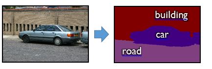
In photographs you could imagine this being used to help selectively edit your photos, or even synthesize entirely new photographs; we’ll see a few more applications in just a minute.
Solving semantic segmentation can be approached in many ways, but one powerful building block is pixel-wise classification: training a classifier to predict a distribution over object categories (e.g. car, road, tree, wall etc.) at every pixel. This task poses some computational problems for ML. In particular, images contain a large number of pixels (e.g. the Nokia 1020 smartphone can capture at 41 million pixels per image). This means that we potentially have multiple-million-times more training and test examples than we had in the whole-image classification task.
The scale of this problem led us to investigate one particularly efficient classification model, decision forests (also known as random forests or randomized decision forests). A decision forest is a collection of separately-trained decision trees:
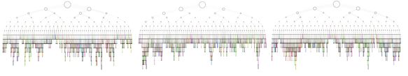
Each tree has a root node, multiple internal “split” nodes, and multiple terminal “leaf” nodes. Test time classification starts at the root node, and computes some binary “split function” of the data, which could be as simple as “is this pixel redder than one of its neighbors?” Depending on that binary decision, it will branch either left or right, look up the next split function, and repeat. When a leaf node is finally reached, a stored prediction – typically a histogram over the category labels – is output. (Also see Chris Burges’ excellent recent post on boosted variants of decision trees for search ranking.)
The beauty of decision trees lies in their test-time efficiency: while there can be exponentially many possible paths from the root to leaves, any individual test pixel will only pass down just one path. Furthermore, the split functions computation is conditional on what has come previously: i.e. the classifier hopefully asks just the right question depending on what the answers to the previous questions have been. This is exactly the same trick as in the game of “twenty questions”: while you’re only allowed to ask a small number of questions, you can quickly hone in on the right answer by adapting what question you ask next depending on what the previous answers were.
Armed with this technique, we’ve had considerable success in tackling such diverse problems as semantic segmentation in photographs, segmentation of street scenes, segmentation of the human anatomy in 3D medical scans, camera relocalization, and segmenting the parts of the body in Kinect depth images. For Kinect, the test-time efficiency of decision forests was crucial: we had an incredibly tight computational budget, but the conditional computation paired with the ability to parallelize across pixels on the Xbox GPU meant we were able to fit [1].
In the second part of this series, we’ll discuss the recent excitement around “deep learning” for image classification, and gaze into the crystal ball to see what might come next. In the meantime, if you wish to get started with ML in the cloud, do visit the Machine Learning Center.
Thanks for tuning in.
Jamie, Antonio and Sebastian
[1] Body part classification was only one stage in the full skeletal tracking pipeline put together by this fantastic team of engineers in Xbox.