How to Hide, Replace, Empty, Format (blank) values with an empty field in an Excel Pivot Table without using filters –Step-By-Step
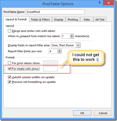
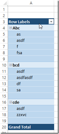
I have been struggling with this for a while. Excel puts the word (blank) on a pivot table field if it does not have any data. I want the field displayed without data. I see in Excel 2013 there is a checkbox under Pivot Table options but I could not get it to work ![]()
I did however finally figure it out. I could solve it using conditional formatting. I many workarounds online in the forums but unfortunately, after a data refresh, the pivot would revert. Using conditional formatting we do not have this problem.
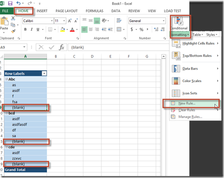
Select the cells that you want to conditionally format [have a (blank) value] (you could select the entire column or even the table too if you want to do multiple columns [even if they do not have (blank) values)
On the Home Tab of the Ribbon Select Conditional Formatting
From the Dropdown, select New Rule
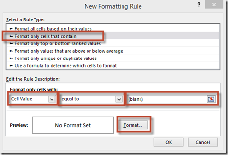
Select Format only cells that contain
In the drop down box box select Cell Value
in the second drop down box select equal to
In the third box type in “ (blank) ” without the quotes
Click the Format… Button
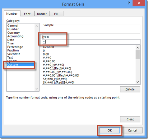
On the Number tab; select Custom
Then to the right, under the word Type: just type in 3 semi-colons “ ;;; ” without the quotes
Click OK
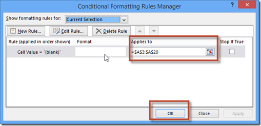
If you want to change anything later (like the range to select the entire column or entire table) you can click Conditional Formatting then Manage Rules
Change the range to whatever you want the range to be and click OK
If you want to delete the rule; click Delete Rule
