How to Analyze your Facebook Data with Power BI
Update 2015-07-30: Facebook changed their API a few months ago. It is now only possible to connect with Power Query to pages you own. Power Query must be approved by the page owner, and once completed, the steps below can be followed.
Update 2015-11-08: The diagram of the Microsoft BI platform has been updated following the general availability of Office 2016, general availability of Power BI, and announcement at PASS Summit 2016 of the Microsoft reporting roadmap. For a forward-looking analysis of the Microsoft visualization tools, please read my new blog post: Positioning of Microsoft Reporting Tools and Roadmap: Excel, Power BI, Datazen, SSRS!
You’ve seen with my last post the types of analytics easily possible with Excel. Now let’s show you how you can make a similar analysis of any Facebook page you like.
Step 0: Getting the tools ready
For this to work, you need Excel 2013 with the Power BI add-ins enabled. Here’s a quick recap of the Microsoft BI platform components:
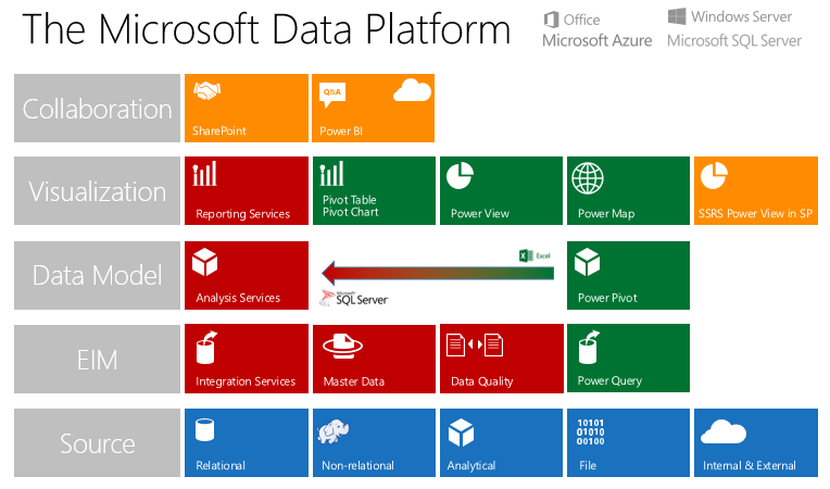
Power Query is the the Excel tool used to access, discover and transform data easily. One of the Power Query connector is Facebook which we will use here. Power Query is a free download for Excel 2010 and Excel 2013. You can download it here.
Power Pivot is a high-performance, in-memory, database engine integrated in Excel since 2010. With this tool you can model your data by establishing relationships, creating hierarchies, adding aggregation business logic, and creating key performance indicators (KPIs). To activate Power Pivot, follow these steps.
Power View is a visualization tool for data exploration to create interactive dashboards as easily as you can create pivot tables. Power View is a new feature in Excel 2013 that must be enabled.
Power Map allows you to see your data on either Bing maps or your custom maps with only a few clicks. Power Map is a ‘bonus’ feature of Office 365 Pro Plus. For other versions of Excel 2013 a preview version is available. Power Map is not required for this analysis.
Step 1: File Preparation
1. The first step is to download the file I posted at the bottom of my last article.
2. You can then replace all the static images, logos on the different tabs.
As an example I’ll be loading data from Cirque du Soleil’s Kurios’ Facebook page.
Step 2: Changing the Data Source in Power Query
Let’s now retarget the query to our new source.
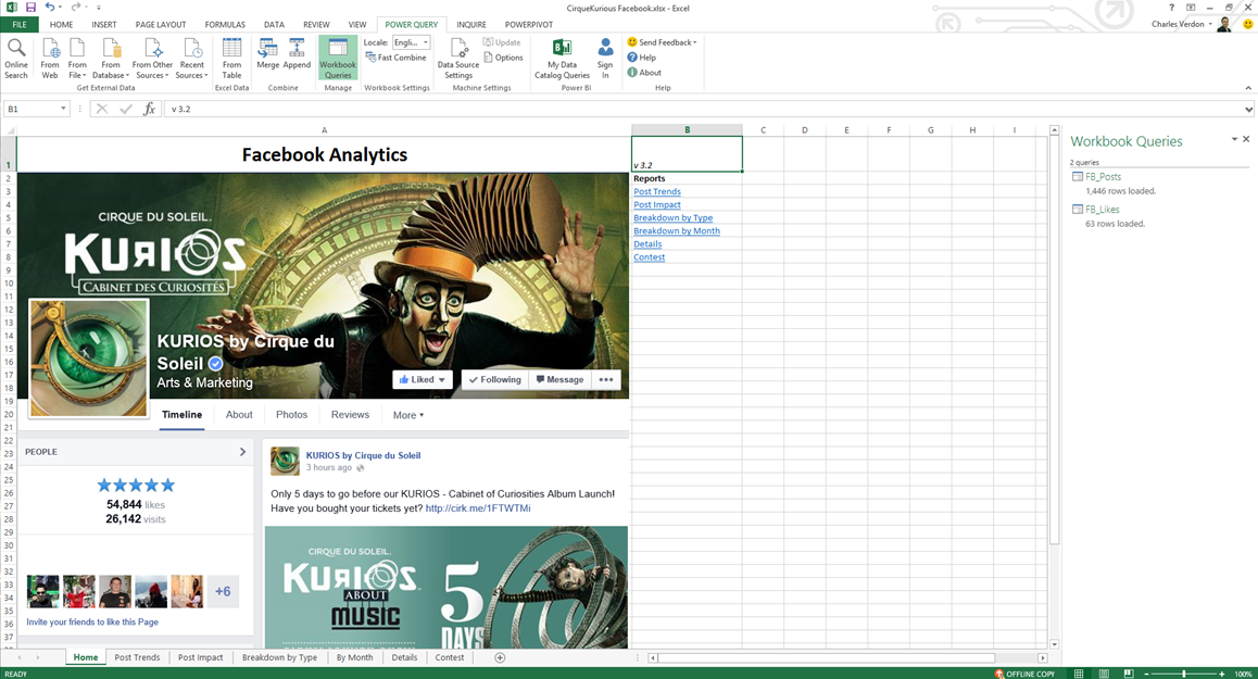
1. Open the list of queries by going on the Power Query tab in the ribbon and selecting Workbook Queries. (See picture above)
2. You will see on the right two queries listed. FB_Posts is the only queries we’re interested; it obtains all the activity on the FB page. FB_Likes obtains all the pages liked by your target page (here Cirque’s Kurios) which is not used in the analysis.
3. Disconnect the load of the FB_Post query by right-clicking, selection Load To and unchecking Load to Data Model. You will get a warning of potential data loss, select continue.
4. The previous steps removes the current data from the Data Model. It is required to avoid the Power Query error of changing a source query after the connection to the model is already made.
5. Double-click on FB_Posts to open the Power Query Editor Window.
6. In the view ribbon, select Advanced Editor. This shows the code view of the query, which is easier to edit than using the Power Query user interface considering the customization done to optimize the load.
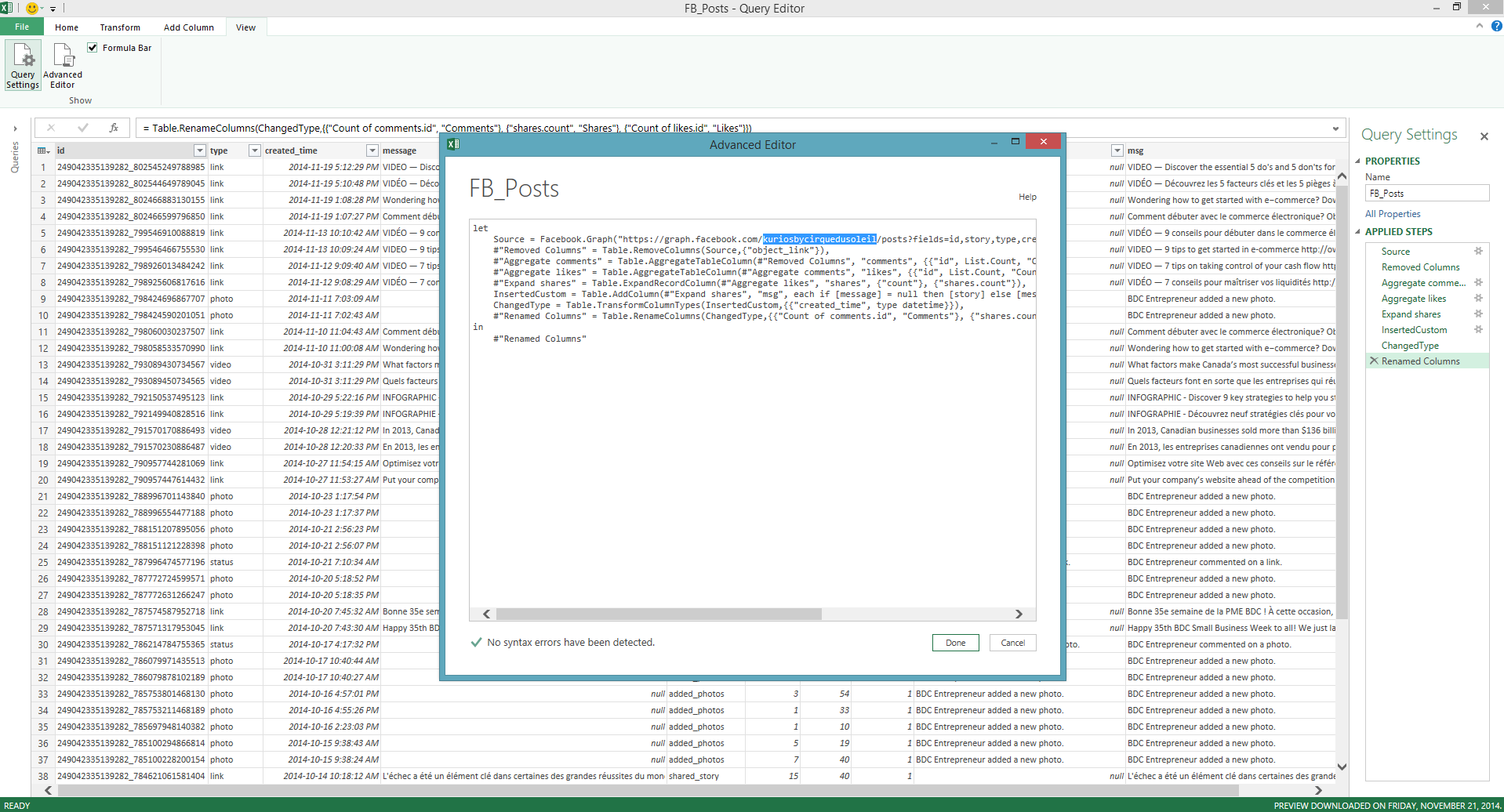
7. Replace the word Microsoft Canada by your target FB page URL as shown above.
8. Click Done and then File and Close & Load.
9. Reactivate the load to the data model by right-clicking on the FB_Posts query and selecting Load To. In the load options select Load to Data Model.
10. Wait until the data is loaded.
Note that it’s possible that you get an error from Facebook saying that you’ve reached your user limit. This is a problem when pages have too much data and retrieving it goes over the Facebook API limit.
Step 3: Update the Data Model
Now that we have the data loaded, let’s update the Power Pivot semantic model.
1. On the Power Pivot ribbon tab in Excel click on Manage.
2. The Power Pivot model window will open. Locate the entity (sheet) FB_Posts and click on this tab.
3. Add a column calculation in the right-most column. The formula should be =date(year([created_time]),month([created_time]),day([created_time]))
4. Rename that column create_date. This will be our link to the date table for the relationship.
5. Likewise, create a column IsContest with formula:
=if(or(FIND("gagne", lower([message]),,-1)<>-1,or(FIND("concours", lower([message]),,-1)<>-1,or(FIND("contest", lower([message]),,-1)<>-1,FIND("win", lower([message]),,-1)<>-1))),"Y","N")
6. Format the Shares column as a Whole Number using the Data Type option in the formatting section of the Home ribbon.
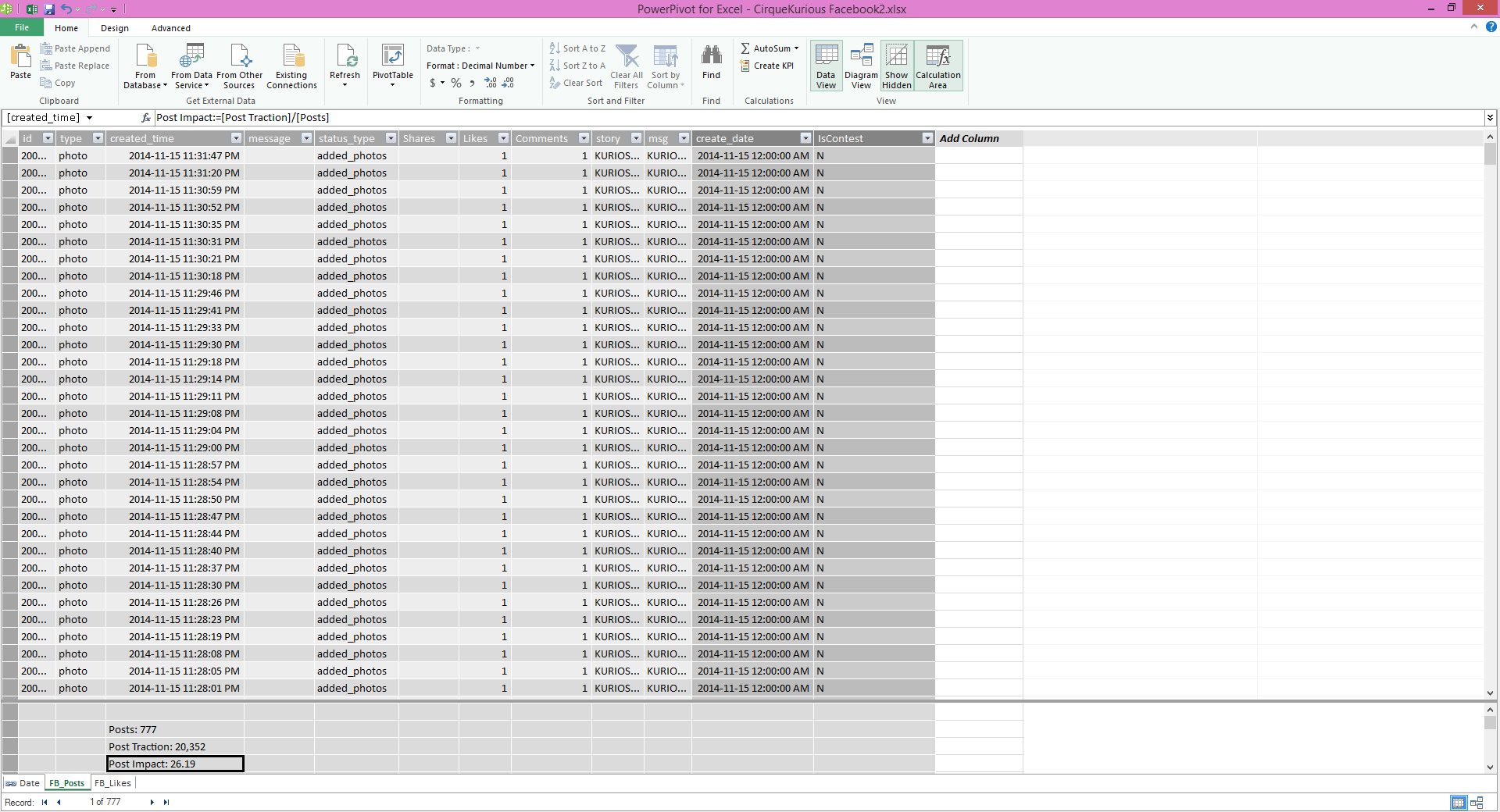
7. In any of the aggregate calculation cells at the bottom of the screen, add the following 3 calculations:
Posts := countrows(FB_Posts)
Post Traction := sum( [Likes] ) + sum( [Comments] ) + sum( [Shares] )
Post Impact := [Post Traction]/[Posts]
8. Format all three calculations in number format either using the format command in the formatting section of the Home ribbon or right-clicking on the cell.
9. The screen should like this:
10. Switch to the relationship view by clicking on the Diagram View button located in View section of the Home ribbon.
11. Drag the create_date column from the FB_Posts table unto the Date column of the Date table. You will see an arrow created.
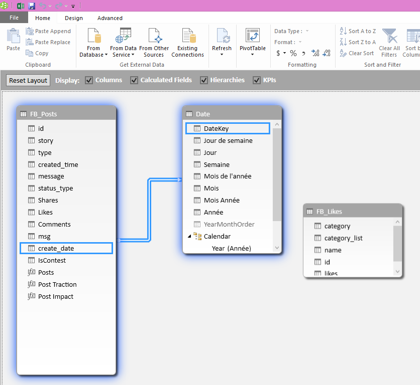
12. That’s it! Close the Power Pivot window.
Step 4: Visualization and Data Exploration
You can then visualize the different tab and play with the data.
It’s usually pretty simple to find a story within the data and then to create new visualizations that further drills down into the questions you have or interesting data points!
Have fun playing with this workbook!
Let me know what you think on twitter! @chverdon